Visual Localization
Visual Localization Based on a Prior Map
Visual Localization In Hdmap
Problem Definition:
Given a high-definition map or environment model, and given a camera (not limited to monocular, stereo, multi-camera, pinhole, or fisheye), output the high-precision camera pose relative to this map. In this process, information from other sensors is optional.
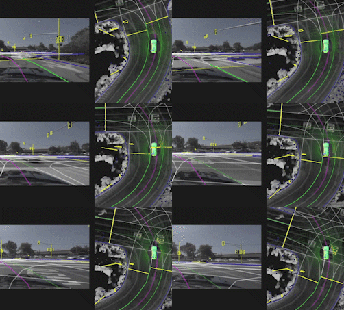
https://news.developer.nvidia.com/drive-labs-how-localization-helps-vehicles-find-their-way/
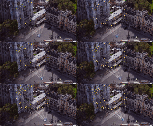
https://github.com/ethz-asl/hfnet
The Relationship Between HD Maps, High-Precision Localization, and Perception
A document from Heduo Technology (HoloMatic) mentions (https://www.zhihu.com/org/he-duo-ke-ji):
HD maps, high-precision localization, and perception complement one another.
If we have an HD map and perception results, we can provide prior information for localization
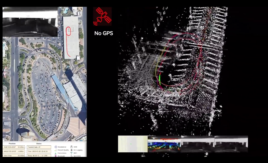 (artisense visual slam preview)
- If we have an HD map and localization results, we can project map elements into the vehicle body coordinate frame to provide prior information for perception
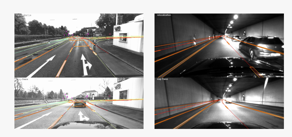 https://www.atlatec.de/localization.html
 - If we have localization and perception results, we can back-project perceived elements into the map coordinate frame, comparing perceived elements with existing map elements to update them or to build a new map
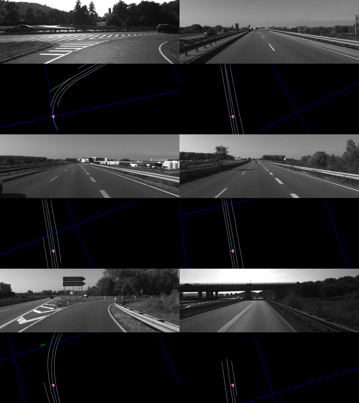
Industry Landscape
- NVIDIA
Domestically it partners with AutoNavi, NavInfo, and Kuandeng, and internationally it partners with TomTom, HERE, Zenrin, and others. DRIVE LOCALIZATION, localization within the world robustly and accuratly https://www.bilibili.com/video/BV1cp4y1e7NM
- Mobileye
Localization in the road book (REM)
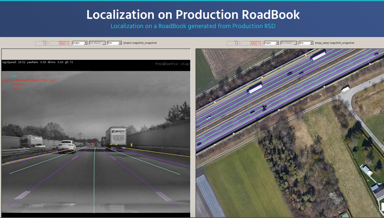
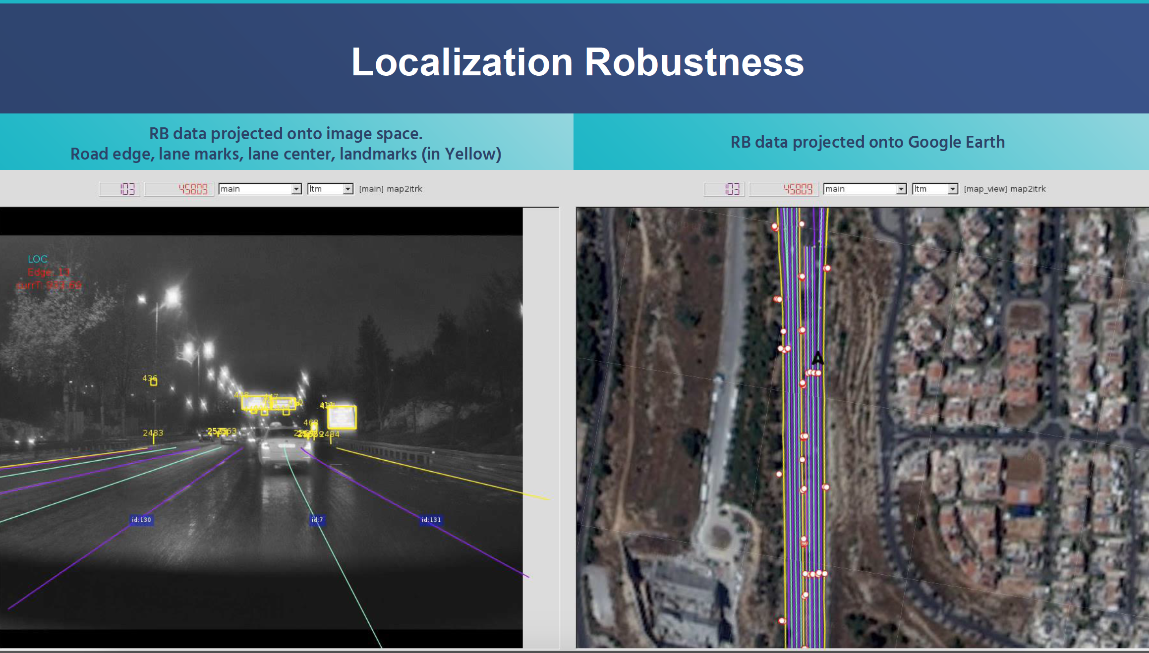
The images above show the results of projecting the road book into image space and onto Google Earth, respectively. Personally, I think that on the one hand Mobileye is an autonomous-driving company, and as its REM system continues to evolve, it may also become a global geographic data asset management company.
http://news.eeworld.com.cn/mp/ICVIS/a77059.jspx
- Baidu
structure based 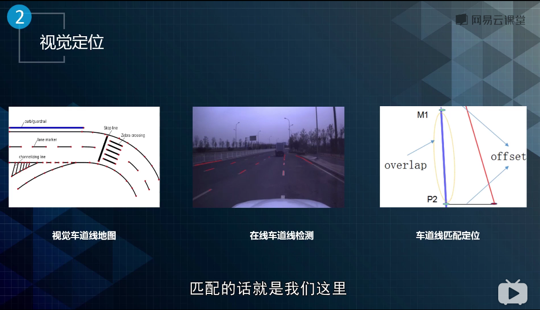 https://www.bilibili.com/video/BV1ib411z7Zx?from=search&seid=12997973010477634399
deep attention based 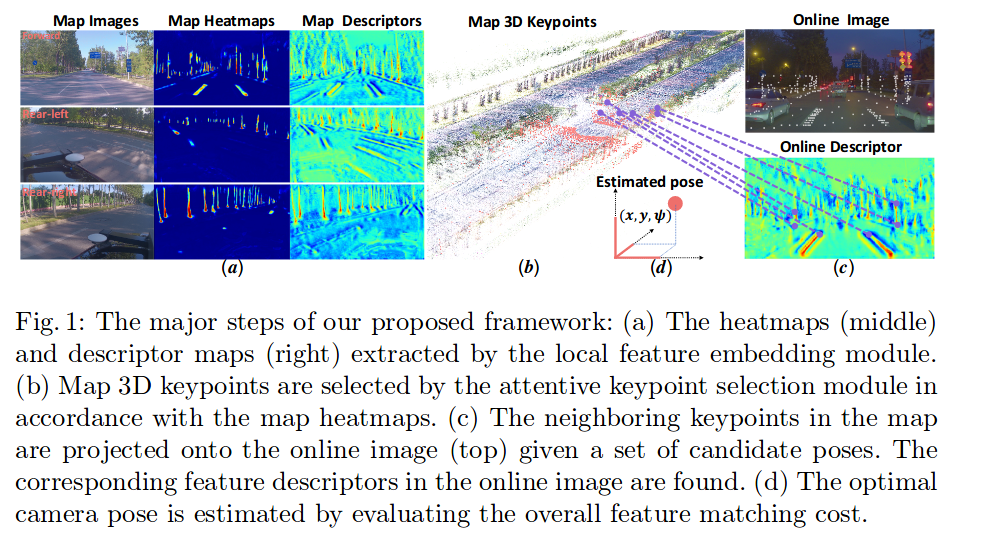 DA4AD: End-to-End Deep Attention-based Visual Localization for Autonomous Driving,ECCV 2020
NIO
Localization accuracy of 20 cm with the support of HD maps https://www.bilibili.com/video/BV1Bf4y1D7Lx- Boash https://www.bilibili.com/video/BV13a4y1a7wk
- GM: Super Cruise https://www.bilibili.com/video/BV1Ba4y1J7Zs?from=search&seid=16396162737053386863
GAC New Energy (Aion V) https://www.zhihu.com/question/395047744/answer/1249197198)
- Momenta
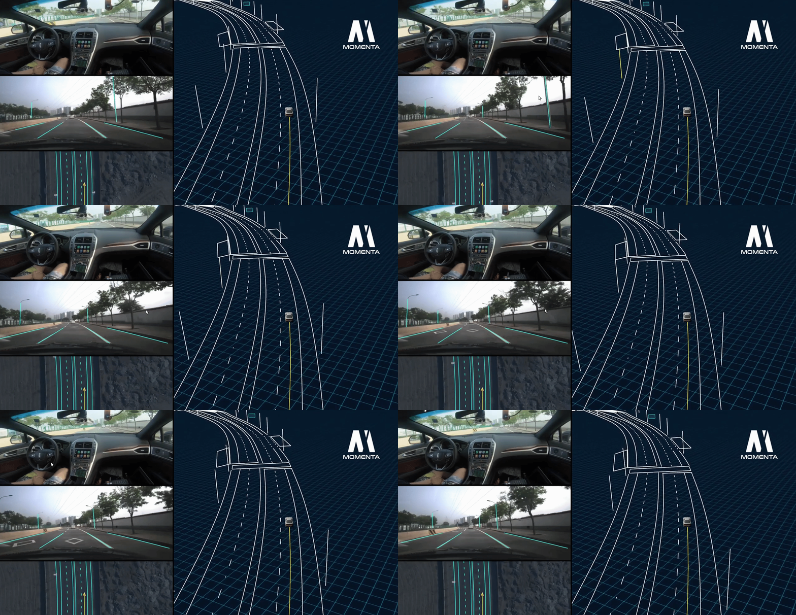 https://www.momenta.cn/our.html
- HeDuo
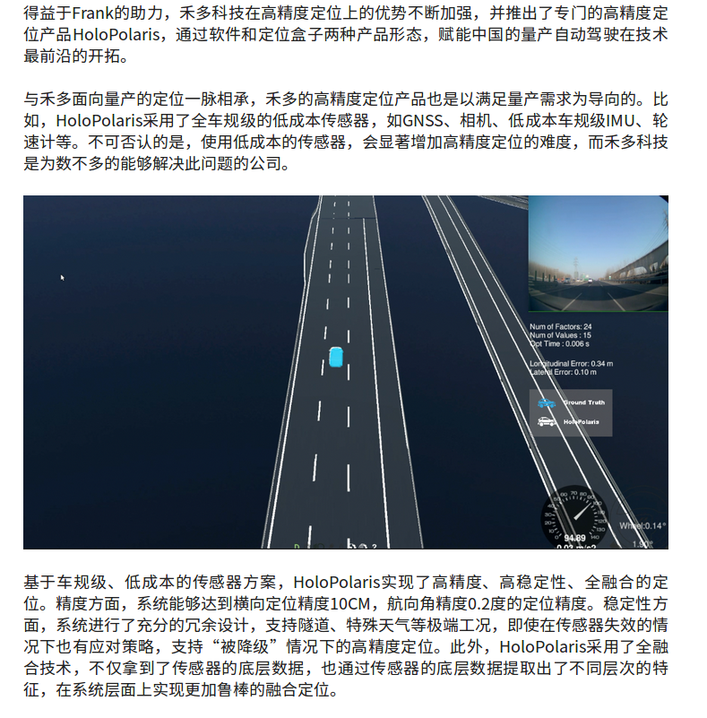 http://www.holomatic.cn/news/read/121.html
Related Paper
Monocular Vehicle Self-localization method based on Compact Semantic Map (2018)
Input: monocular camera + map. Output: 6-DOF pose. The overall pipeline is as follows:
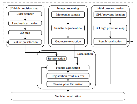
Intermediate results: 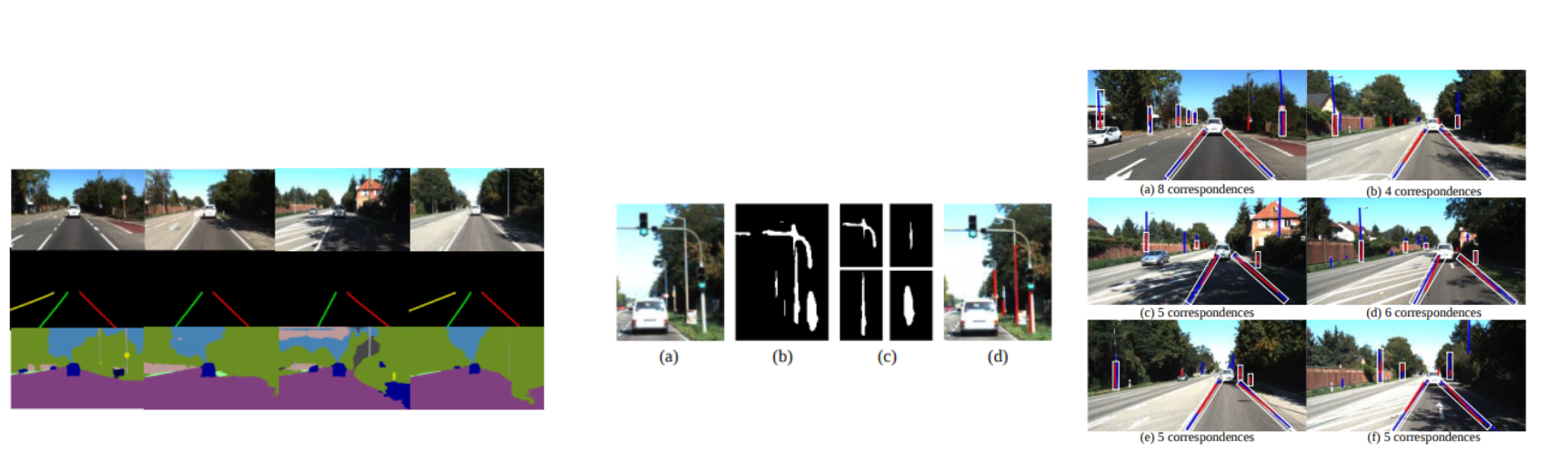
Data association is established through map projection. Localization result: KITTI odometry dataset sequence 4: 0.345 m
Monocular Localization with Vector HD Map(MLVHM): A Low Cost Method for Commerial IVs (2020)
This paper proposes a localization method that couples a monocular camera with a lightweight vector map. It establishes associations between map features and the relatively stable semantic features detected in images, thereby estimating the camera pose. At the same time, to add constraints and make the trajectory more robust and smooth, it introduces visual-odometry constraints between two frames, ultimately achieving a localization RMSE accuracy of about 24 cm.
As is well known, GNSS-RTK + a high-quality IMU + a multi-beam LiDAR can deliver high-precision localization results both indoors and outdoors, but this cannot be commercialized at scale due to cost. The authors’ team therefore hopes to accomplish this task using only a monocular camera + an HD map. Although the HD map itself needs to be built with expensive sensors, some companies do use crowdsourcing techniques so that consumer-grade sensors can be used to build and update maps. Moreover, once a map has been built, its marginal cost approaches zero; it is distributed through the cloud, and the more vehicles it is distributed to, the lower the amortized construction cost per vehicle. The forms of maps used in autonomous driving are also varied, as shown in the figure below: there are LiDAR point-cloud maps containing the raw geometric information of the environment that are needed for LiDAR localization; there are feature-point maps such as those built in feature-based visual SLAM; and there are vector maps that provide a topological representation of the environment, similar to the one in the right figure. All of these maps can accomplish the localization task. Considering the requirements of map size and compactness, a vector map may be a more suitable choice, and it is the one used in this paper. Of course, for one and the same vector map there exist many format standards internationally, such as OpenDRIVE, Apollo, NDS, and so on. Two different forms of maps are shown below:
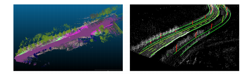
Because changes in illumination, viewpoint, occlusion, and so on occur frequently in outdoor environments, it is necessary to select, from the environment’s features, those that are more robust to these conditions. Leveraging the extremely strong representational power of CNNs on images, we can obtain the pixels or descriptors where these stable semantic features are located, and what is stored in the vector map is likewise these invariant, relatively stable things. The problem therefore naturally reduces to a data-association problem. The overall pipeline of the method proposed in the paper is as follows:
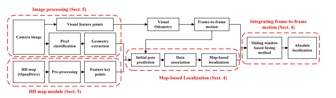
Unlike the previous work, it simultaneously solves the frame-to-frame VO (using the traditional visual feature ORB) and introduces frame-to-frame constraints in a sliding window to improve robustness.
In the image-processing module, key pixels are extracted through segmentation and fitted into point features (signs) and line features (lanes and poles); at the same time, ORB features are extracted in order to compute the frame-to-frame VO. In the map-based localization module, an initial pose is estimated, and using this initial pose the optimal matches are determined by random sampling; the pose can then be optimized and solved based on the matching relationships. Finally, to ensure robust localization output, sliding-window pose optimization is added.
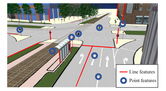
Definition of the residual: for a point feature, it is simply the most basic point reprojection error; for a line feature, it is the distance from the projected point of a map line to the line segment detected in the image. (For the residual, the approach we currently adopt here should be more advantageous: 1. it unifies the description of all features, describing them all with points; 2. it does not require explicit data association.)
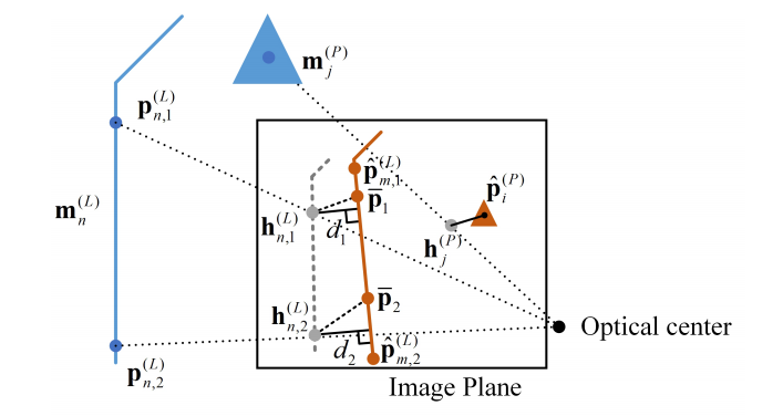
The data-association process: determining the correspondences between features on the map and features in the image
- First generate a set of possible correspondences, then randomly sample from this set the correspondences of three line features with the same semantics to compute the camera pose,
- Project the map elements according to the computed camera pose; if the distance to an image feature is below a set threshold, it is regarded as an inlier. The distance between the estimated pose and the initial pose is then computed, and if it satisfies the threshold, the correspondence is added to the hypothesis set
- Finally, select the group of correspondences with the largest number of inliers as the final correspondences
Coupling frame-to-frame pose constraints (pose fusion) An optimization problem is constructed in which the state variables include the pose and scale of each frame. The state variables are solved by combining the scale-less frame-to-frame constraints given by monocular ORB-SLAM with the map-localization result of each frame. The energy function is as follows:
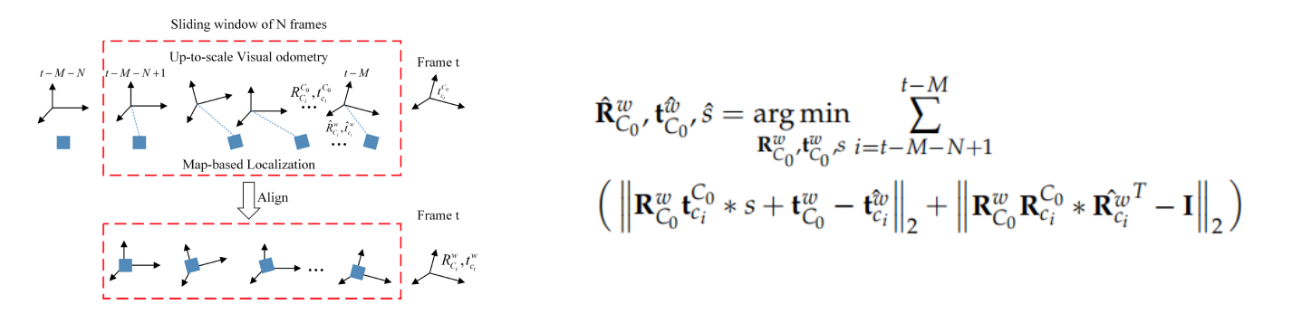 Solve for the rotation, translation, and scale of the first VO frame relative to the map, aligning the VO poses with the map-based localization poses
Implementation details:
- At the image-feature-extraction level, a modified version of PSPNet is used to segment the image; specific pixels are then selected according to their confidence probabilities and partitioned into different regions using region growing. Line features are fitted by least squares, point features are fitted from sign regions, and the positional description of each of these features is obtained in the image domain
- Use of the compact map: the map used is in OpenDRIVE format. Signs use their centroid point, poles use their two endpoints, and lanes are sampled into discrete points at 0.2 m intervals, with every two adjacent points fitted into a line for use
- Optimization and initialization: system initialization also uses low-cost GNSS measurements as the initial value, and the optimization is the standard LM algorithm
Experiments:
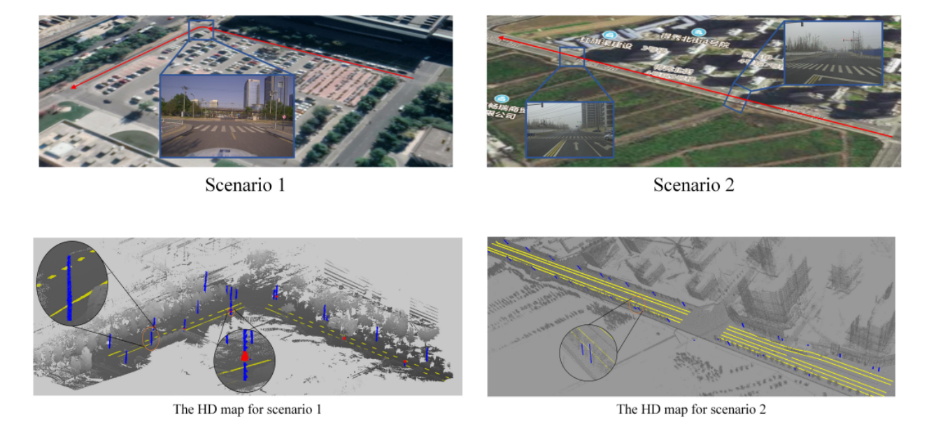
These are a campus scene and an external road scene, respectively. First is the map generation for the corresponding scene: LOAM is used to generate the road point-cloud map, then lane lines, poles, and signs are extracted manually (we did something similar last year), and the corresponding OpenDRIVE-format vector map is then generated, at about 50 KB per kilometer, whereas the corresponding point-cloud map is about 600 MB per kilometer. The map accuracy verified with a total station is about 9.25 cm
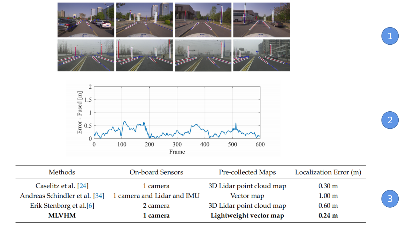
- The projected matched features 2. The localization error after fusion 3. Comparison of localization accuracy with other methods
HDMI_LOC: Exploiting High Definition Map Image for Precise Localization vai Bitwise Particle Filter (IROS 2020)
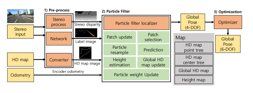
This paper proposes a method that combines a stereo camera with an HD map to perform 6-DOF pose estimation. It converts the map into an 8-bit image representation so that the query image can be matched against the map through bitwise operations, and it uses a particle-filter framework for pose optimization and estimation. Under an 11 km test condition, the lateral and longitudinal errors are about 0.3 m, and it runs at 10 Hz. The entire localization process can be divided into four steps:
- Image-processing step: obtain a semantic segmentation map and a disparity map from the stereo images (which is why this method is relatively slow)
- Convert the HD map into an 8-bit image
- Use a particle filter to estimate the 4-DOF (three translations + yaw) pose using the patch of the current image and the map image; because both are 8-bit images, a bitwise-AND operation can be used for fast computation
- Estimate the full 6-DOF pose by additionally computing roll and pitch through optimization
The overall pipeline is as follows:
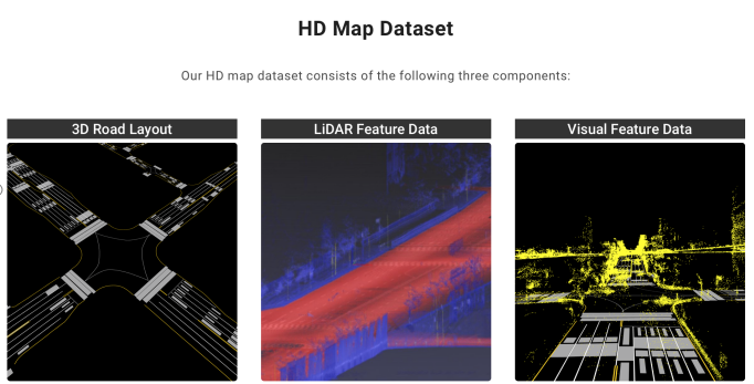
The map directly adopts the vector-format HD map published by Naver Labs (a Korean autonomous-driving organization, https://hdmap.naverlabs.com ), stored as a shapefile. The map includes features such as lanes, stop lines, and ground signs
- Conversion of the vector map into an image:
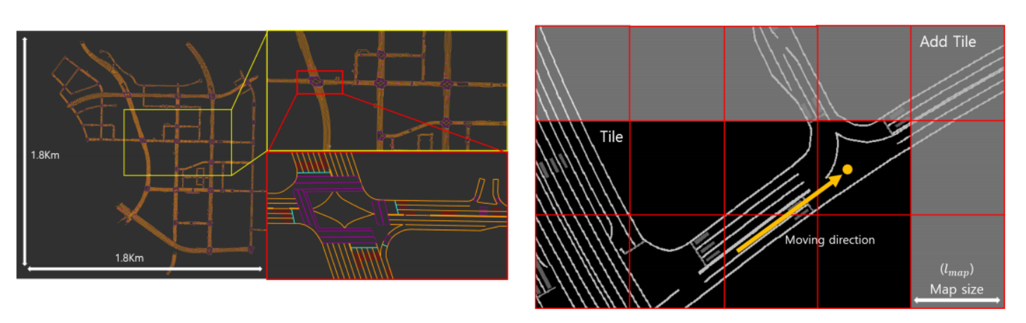
Gray-scale values of 128, 64, and 32 represent lane lines, stop lines, and road signs, respectively. Each tile is 30 m * 30 m and stores the coordinates of its corresponding center point in the global UTM coordinate system. Preprocessing and 8-bit representation: the figure above shows a global HD map image, which is extended according to the current vehicle pose. In the preprocessing step, an HD map center tree and an HD map point tree are generated at the same time. The center point makes it easy to look up nearby tiles, while the point tree is composed of the set of points in the shapefile and is used to find the nearest point in order to obtain height
- Conversion of stereo images into a point cloud: Stereo images generate a labeled point cloud: OpenCV stereoBM generates the disparity map, and combining it with the CNN semantic segmentation map, a labeled point cloud can be easily obtained
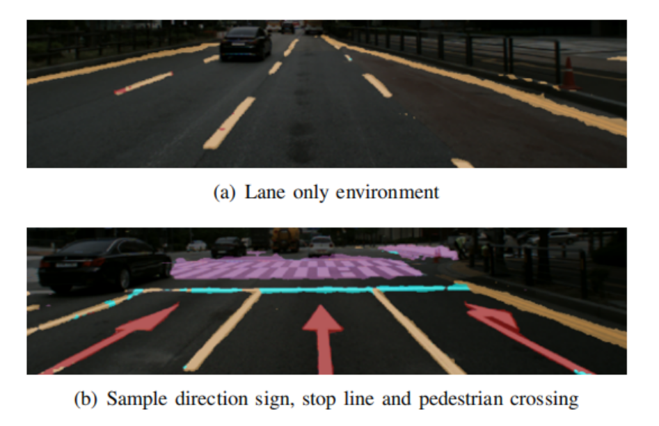
- On the maintenance and selection of patches: For each newly entering subpatch, the latest current patch is updated or a new patch is added according to the current situation. When updating a patch, the semantic coordinate points in the stereo-camera coordinate frame are first transformed into the world coordinate frame, and then the points in the world coordinate frame are projected onto the patch image:
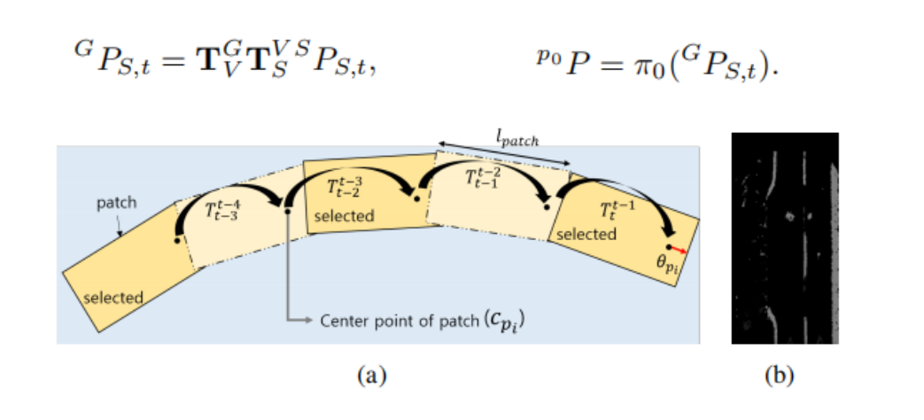 In this way the new information is added onto the most recent patch image. If the most recent patches already exceed five, a new patch is built from the current subpatch. At the same time, each patch records an age; as new patches are added, the age of older patches decays, and this is later reused as the weight of the patch during the particle-filtering process
On patch selection: ultimately these patches are matched against the map. To be more computationally efficient, the most informative patches are used to compute the matching score; for example, a patch that contains lanes, poles, and road signs at the same time is more important than a patch that contains only two lanes. Finally, based on a set threshold for each type of landmark, some of the more important patches are selected
- Particle filter
The purpose of the particle filter is to estimate the current vehicle’s 2D pose (tx, ty, yaw). Because it uses the matching of two planes, the patch and the tile, it can only estimate a 2D pose; the height is obtained directly by looking up the height of the nearest point. Thus the final output of the particle filter is a 4-DOF pose of the form (tx, ty, tz, yaw)
The process includes:
Particle resampling
Particle prediction: propagate the particles according to the motion model with added Gaussian noise
Obtain the candidate tile set according to the current position
Update the particle weights using the AND operation
From the result image of the AND operation, the numbers of lane, stop-line, and sign pixels can be obtained; the larger these numbers, the better the current pose estimate, and correspondingly the higher the particle weight
- Finally, take the average pose of the top 3% of particles with the highest weights as the final pose
- Estimating roll and pitch by optimization Its core is to construct a residual such that, when the vehicle’s roll and pitch change, the residual produces a corresponding continuous change. The steps are as follows:
- First transform the stereo point cloud into the vehicle body coordinate frame
- Fit a plane by RANSAC from the points in the vehicle body coordinate frame, obtaining the plane-equation parameters nt = (nx, ny, nz, dt)
- Transform the points in the HD map into the vehicle coordinate frame (which requires the current vehicle pose), and take the distances of these points in the vehicle coordinate frame to the plane as the residual
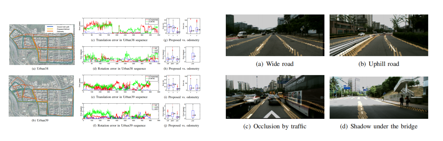
Experimental results:
From Coarse to Fine: Robust Hierarchical Localization at Large Scale (CVPR 2019)
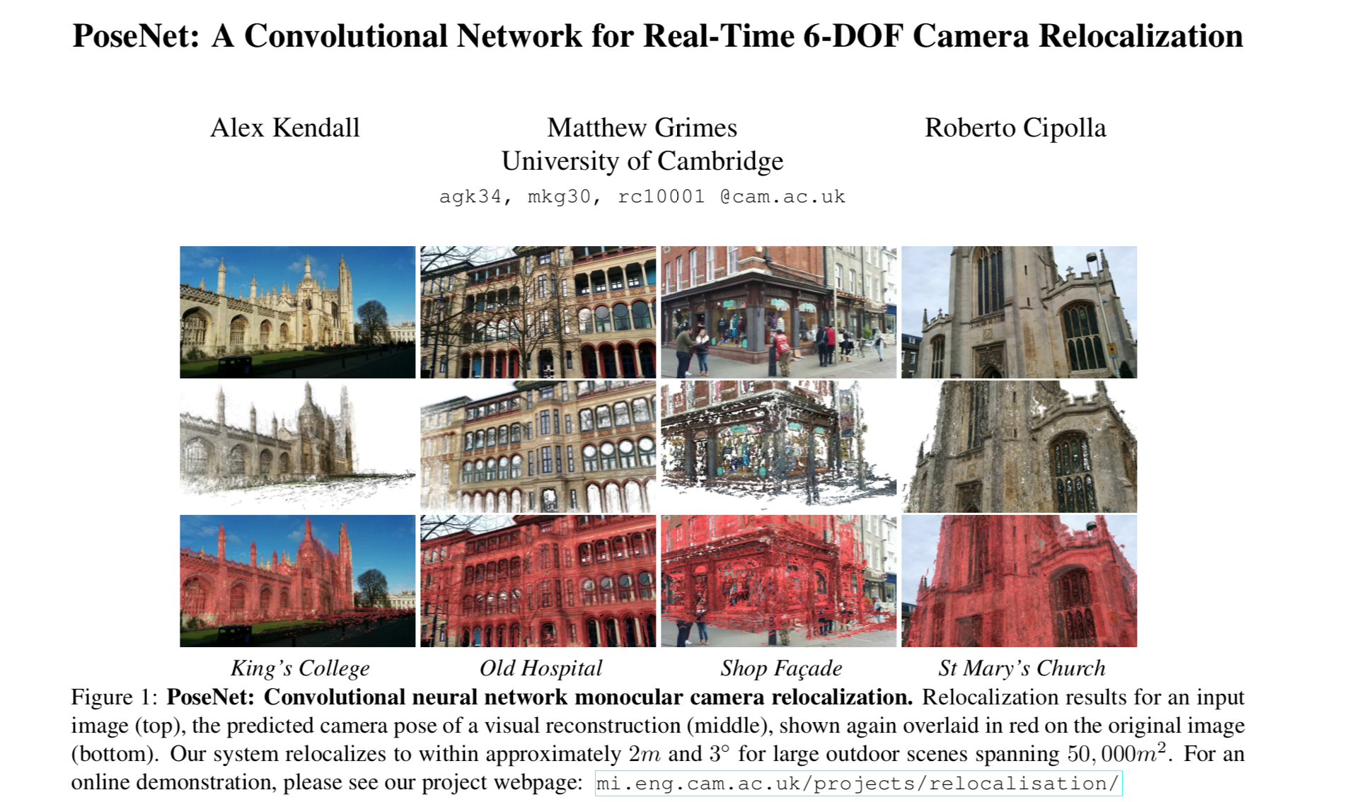
Visual localization refers to computing the pose corresponding to an arbitrary given image, in a large-scale scene where the environment map is known. In the field of visual localization there are basically two main directions. One is the so-called end-to-end approach, whose representative work is PoseNet; such methods directly use images and ground-truth poses as supervision for learning, and for a given image of the same scene they can regress the 6-DOF ground truth. The advantage of this approach is that the database is very small, a single network can cover a very large scene, and although ground-truth poses are needed, no explicit spatial 3D reconstruction is required. But its drawbacks are also obvious: such methods do nothing more than establish a mapping between images and poses through learning, which is essentially a process of image-similarity matching, and therefore they cannot regress precise ground truth or acquire the ability to transfer to unlearned scenes. The currently more popular approach is coarse-to-fine two-step localization. First the closest key frame is found through image retrieval, and then local features are matched with that key frame. Because the key frame’s pose is known, the current frame’s pose can be estimated through methods such as PnP. Two-step localization avoids the time complexity of directly matching among all key frames, and at the same time avoids the space complexity of loading the entire environment map into memory. This paper primarily proposes a coarse-to-fine hierarchical localization network, HF-Net. For an input query image, a single CNN simultaneously predicts the image’s local and global features to perform precise 6-DOF localization, adopting such a coarse-to-fine localization paradigm: candidate frames are first obtained through a global retrieval, and then local-feature matching is performed with the candidate locations to carry out localization. Similar to the way humans localize themselves, the authors hope to use such a coarse-to-fine localization paradigm, while also hoping to combine some advances of deep learning in the field of image feature detection and description; these learned detectors and descriptors improve robustness to environmental changes. To achieve the above goals and maximize efficiency, HF-Net (hierarchical feature network) is proposed, which simultaneously estimates local and global features and maximally shares computation. The network is trained by means of multi-task distillation
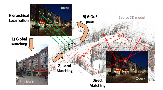
One is a global-then-local approach, and the other performs direct matching based on descriptors
Similar to the way humans localize themselves, the authors hope to use such a coarse-to-fine localization paradigm, while also hoping to combine some advances of deep learning in the field of image feature detection and description; these learned detectors and descriptors improve robustness to environmental changes. To achieve the above goals and maximize efficiency, HF-Net (hierarchical feature network) is proposed, which simultaneously estimates local and global features and maximally shares computation. The network is trained by means of multi-task distillation
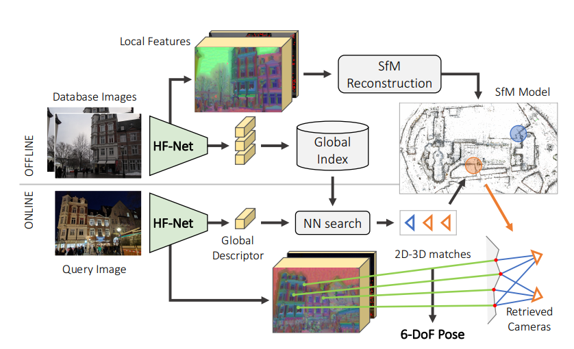
In offline mode, the network is used to extract local and global features from the database images. The local features are fed into an SfM 3D-reconstruction framework to build the environment model, and the global features build a reference-image index database. Then, during online operation, the same feature-extraction operation is performed on the query image; candidate frames are obtained by NN search based on the global descriptor, correspondences are established between the map points co-visible in the candidate frames and the feature points of the query image, and the pose is solved using a RANSAC + PnP framework
The structure of HF-Net:
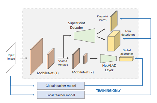
Its architecture contains a single encoder and three predicting heads, namely the keypoint score, the dense local descriptors, and the global descriptor shown in the figure. The sharing of computation shown in the figure is also fairly natural: we know that the global description of an image can be obtained by aggregating local features (for example, the generation of the DBoW bag-of-words used in ORB-SLAM), so the decoder part responsible for feature extraction at the beginning shares parameters. Its decoder part is a MobileNet backbone; to extract the global descriptor, a NetVLAD layer is attached to the last feature map of the MobileNet, and for local-feature extraction, a SuperPoint decoder is attached to obtain the keypoints and local descriptors
For the local-feature branch, local features are more in need of localization accuracy in the image and have a higher requirement for spatial resolution but a lower requirement for semantic features, which is the opposite of the global description; therefore, to preserve spatial resolution, the local-feature branch is established (branches off) earlier
Details of the network architecture: 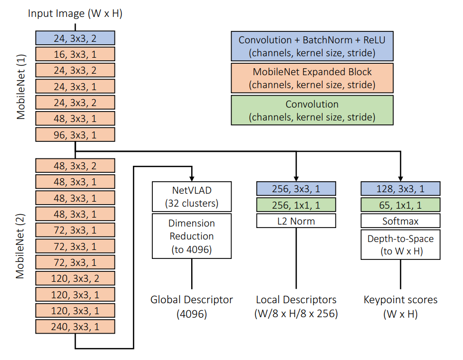
- On the training process Because of issues with the data—data scarcity (it is difficult to obtain the ground truth corresponding to features) and data augmentation (augmentation breaks the global consistency of the image, which makes it difficult to learn the global description)—the authors adopt a multi-task distillation approach to train the network. The core idea is to find some off-the-shelf teacher models to guide the learning of the student model. The loss is as follows:
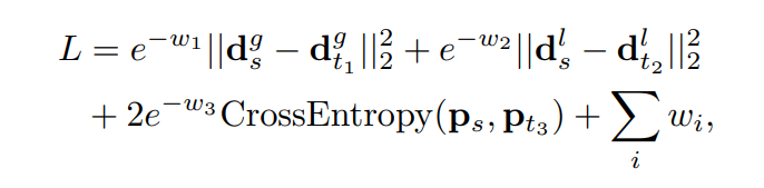
The teachers are treated as ground truth for training. These are, respectively, the L2-norm loss of the global descriptor, the L2-norm loss of the local feature descriptors, the cross-entropy loss of the keypoint score, and the regularization loss of the optimization variables w. The student is a single one, learning from different state-of-the-art teachers; here three teachers, t1, t2, and t3, are brought together, ultimately demonstrating the effectiveness of knowledge distillation on multiple tasks. w1, w2, and w3 are weights that need to be learned automatically
The authors adopt a knowledge-distillation approach. Simply put, the results obtained from training a large network model that has already been shown to be effective are used as the supervisory signal for a small network model, ultimately achieving the effect that the small network model approximately imitates the large network. The hope is to be as accurate as the large network while also being as efficient as the small network
On the choice of teachers:
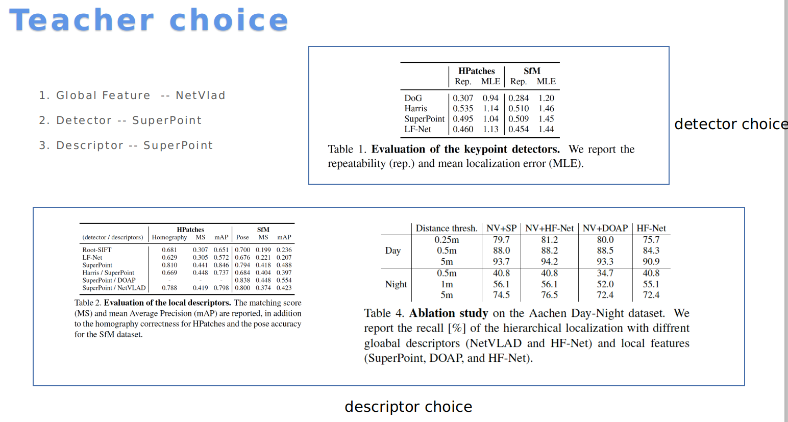
NetVlad & SuperPoint
- Some results of local feature detection
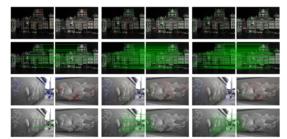
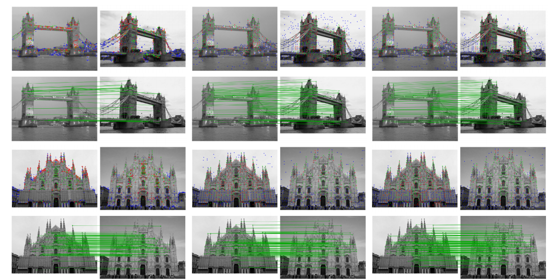
Green marks features that are repeatedly detected, red marks features that are not repeatedly detected, and blue marks features that are not seen in the other image. The figure shows inlier matches; from left to right they are SIFT, SuperPoint, and HF-Net
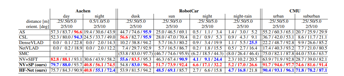
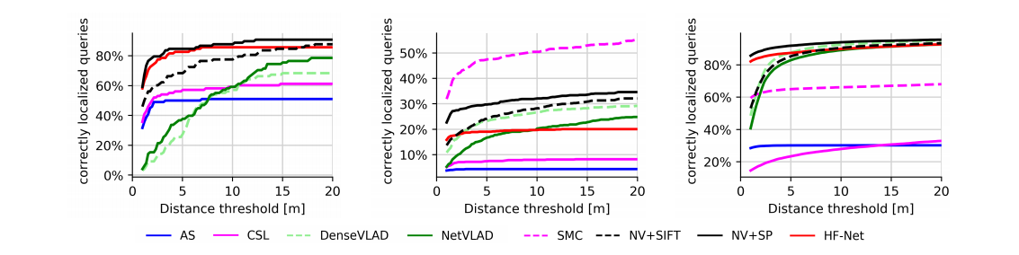
- Localization experiments Experiments are conducted on three datasets: the Aachen Day-Night dataset (a small European city), the RobotCar Seasons dataset (an urban dataset spanning multiple city blocks), and the CMU Seasons dataset (8.5 km of urban and suburban areas). Each dataset has its corresponding database images and query images.
Because an SfM model needs to be built when performing PnP, the basic process is as follows:
- Use the extracted features to perform 2D-2D matching between reference images, and apply an initial ratio-test match filtering
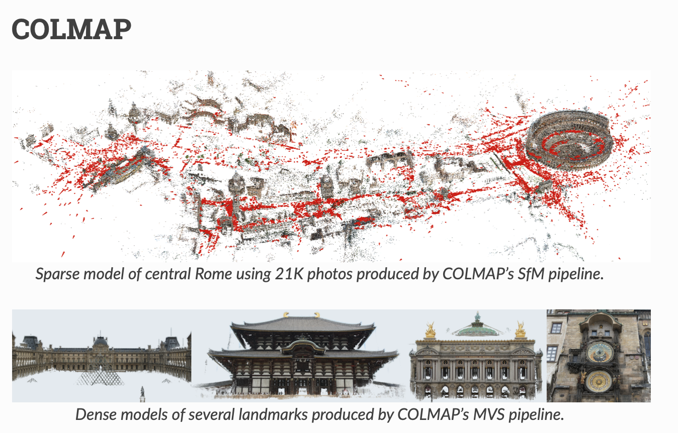
- Use two-view geometry to further filter the matches within the COLMAP framework
- Triangulate based on the matching relationships and the ground-truth poses of the reference images to generate the 3D model of the environment
Statistics of successfully localized frames:
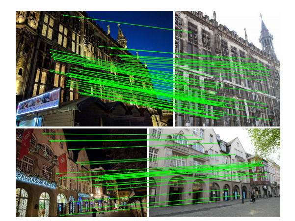
Successful localization results on the Aachen Day-Night dataset. The left figure is the query frame, and the right figure is the retrieved database image with the most inlier matches; the number of inliers is obtained through PnP RANSAC
Runtime analysis:
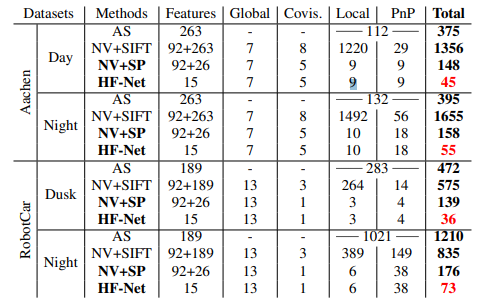
Statistics of the time spent on the different steps; it is more than 10 times faster than Active Search, the currently fastest method
- Some localization results
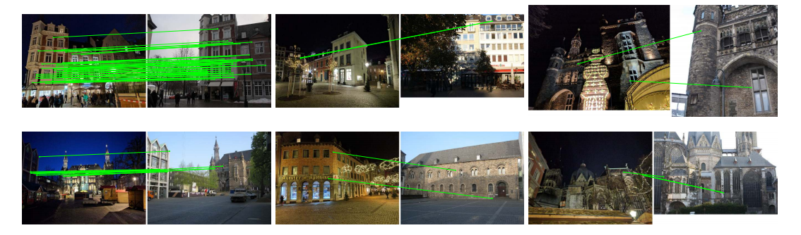
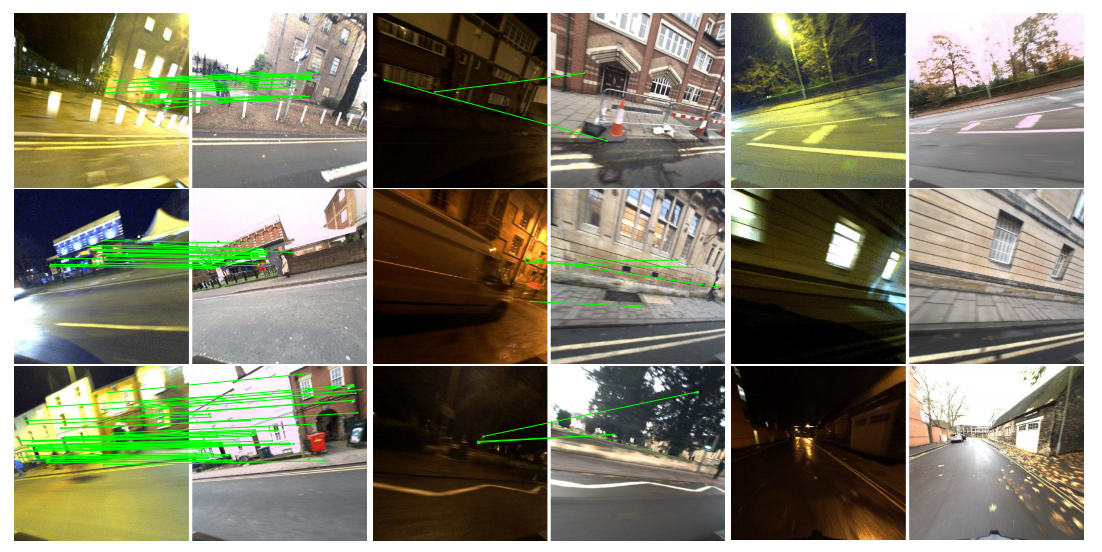
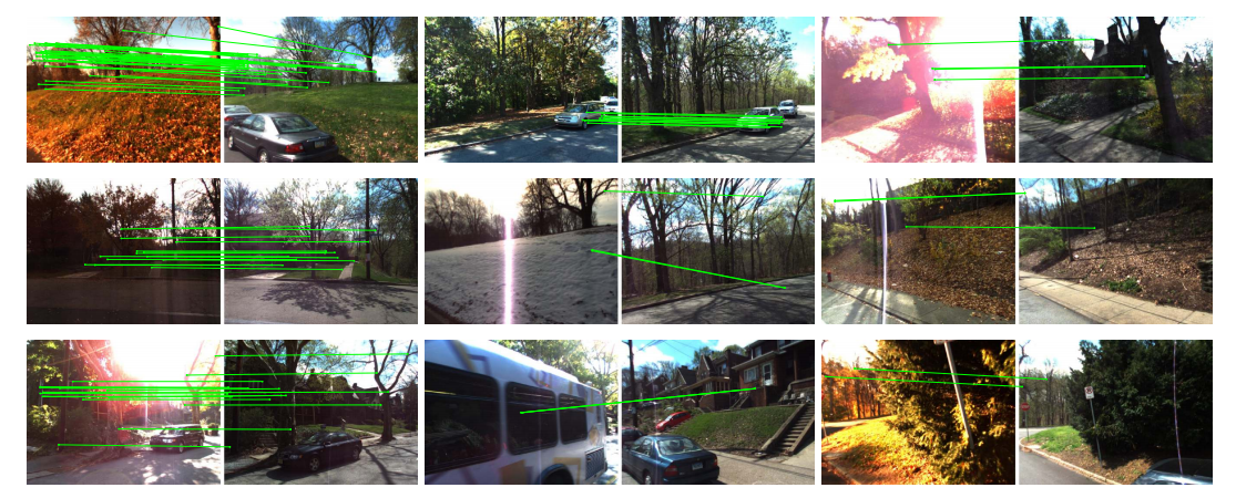
For each image pair, the left is the query image and the right is the retrieved image with the most inlier matches. The left is a case of successful localization under challenging conditions, the middle is a failure caused by an incorrect global retrieval, and the right is a failure caused by insufficient local matching
Comparison with NetVLAD + SIFT:

Compared with SIFT, there are slightly fewer matches, which reduces the computational cost of local matching; at the same time, there are more inlier matches, which improves localization robustness and reduces the requirement on the number of RANSAC iterations
The above is a brief summary of visual localization. If you have any questions, feel free to contact me
cell phone: 13162517010
email: candyguo_fly@163.com
If you find this blog helpful, please consider sponsoring me, so that I can be more motivated to keep updating the blog

Comments