Stereo Match

Stereo Matching

Within the scope of stereo matching, this article focuses mainly on the following two small parts:

Principle analysis of SGM (a classic algorithm)
comparation with monodepth

SGM

The Semi-Global Matching (SGM) algorithm is one of the most popular algorithms in real-time stereo vision, and it has already been widely deployed in many products. It was first proposed by H. Hirschmuller in a paper published at CVPR in 2005
‘Accurate and efficient stereo processing by semi-global matching and mutual information’
Before the strong rise of deep learning algorithms, stereo matching algorithms could be divided into three major schools: the local school (SAD, SSD, NCC, Census-Transform, Mutual Information …), the global school (Graph Cut, Belief Propagation, Dynamic Programming …), and the semi-global school (SGM). SGM is the representative work of the semi-global category. Compared with the crude simplicity of the local school, SGM is more elegant and sophisticated, while not being as time-consuming as the global school (https://blog.csdn.net/rs_lys/)
The SGM algorithm has many steps and is fairly complex overall. I hope that through this sharing, you can gain a better understanding of its principles.
- OpenCV interface
```
cv::Ptr<cv::StereoSGBM> sgbm = cv::StereoSGBM::create(minDisparity, numDisparity, SADWindowSize, p1, p2, diso12MaxDiff,preFilterCap, uniqueRatio, speckleWindowSize, speckleRange, fullDp);
cv::Mat disparity_sgbm;
sgbm->compute(frame->left, frame->right, disparity_sgbm);
disparity_sgbm.convertTo(frame->disparity, CV_32F, 1.0 / 16.0f);
```
Explanation of the parameters:
1. minDisparity: the minimum disparity
2. numDisparity: the number of disparities (64 / 96 / 128 / 256 …)
3. SADWindowSize: the window size used for intensity correlation (3 / 5 / 7 …)
4. p1, p2: smoothness penalty coefficients; their detailed meaning is introduced below
5. diso12MaxDiff: the maximum allowed difference in the left-right disparity check
6. preFilterCap: the truncation value for pre-filtered image pixels (not used below); it is mainly an image pre-processing operation, used to remove noise interference and improve the distinguishability of boundaries
7. uniqueRatio: the uniqueness ratio (ratio test)
8. speckleWindowSize: the maximum size of smooth disparity regions (filters out some speckle noise)
9. speckleRange: the maximum disparity variation within a connected component (speckle)
- reference: (docs.opencv.org)
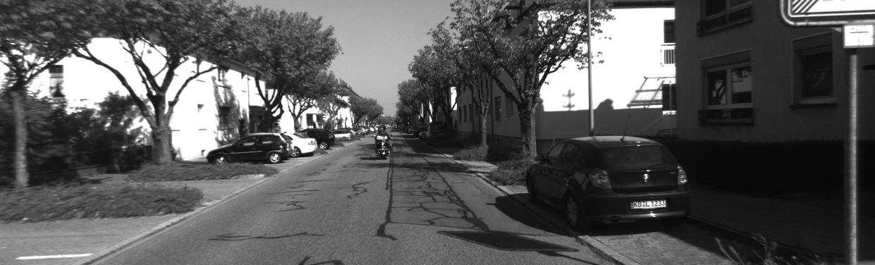
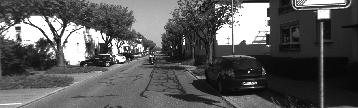
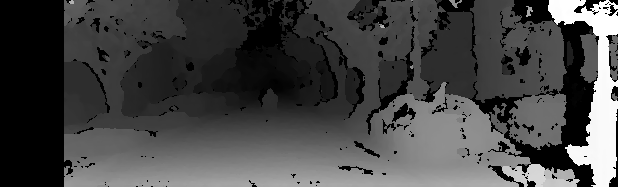
** Example stereo input and output:
left
right
gray-scale show
color map show

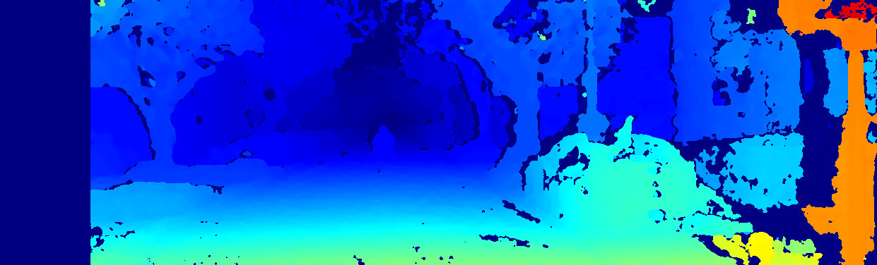
As can be seen, there are quite a few holes and disparity discontinuities. A normal pipeline also includes a disparity-map filtering post-processing step (weighted least squares filtering)

OpenCV interface

wls_filter = createDisparityWLSFilter(left_matcher);
wls_filter->filter(left_disp,left,filtered_disp,right_disp);

After applying the filter:

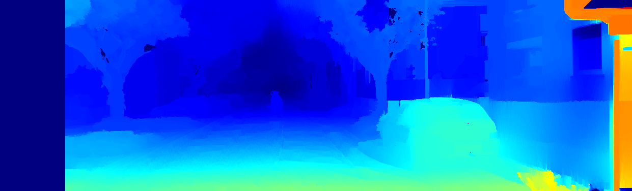
Reference: “Fast Global Image Smoothing Based on Weighted Least Squares”. The gist is that it uses a weighted least squares algorithm for optimization, making the image globally smooth while preserving edges. Its overall functionality is close to that of bilateral filtering. As can be seen, after post-processing the disparity map is smoother and the contours are clearer

Using the open-source monodepth, trained without any parameter modification, and then inferring the depth result corresponding to the image above (https://github.com/OniroAI/MonoDepth-PyTorch):

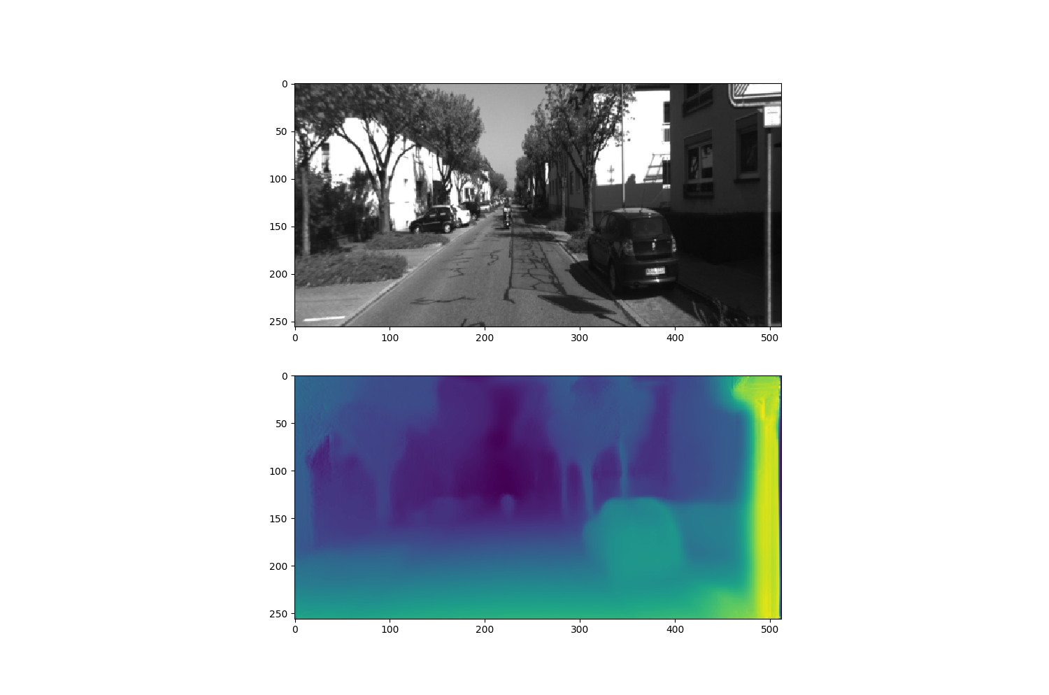
As can be seen from the figure above, in terms of overall performance the deep learning method is superior to the traditional method (The overall performance outperforms by a larger marjin then traditional SGM method)

The overall SGM algorithm pipeline is as follows:
1. Census-Transform: convert the original image into a census image, to facilitate matching cost volume computation
2. Compute-Cost: perform the initial matching cost computation using the two census images
3. Cost-Aggregation: cost volume aggregation, the ‘key step’
4. Compute-Disparity: compute the disparity value of each pixel based on the aggregated cost volume
5. LR-Check: left-right disparity consistency check (optional)
6. Remove-Sparkles: remove scattered speckles (optional)
7. Fill-Holes: hole filling (optional)
8. Middle-Filter: median filtering for denoising and smoothing
Here steps 1-4 are the basic steps, and steps 5-8 are the disparity optimization steps.

Each step is explained in turn below:

census transform Hirschmuller originally chose MI (mutual information) as the matching cost, but compared with the census transform its computational efficiency is relatively low, so the mainstream approach became the census transform. The so-called census image is obtained by transforming the original image pixel by pixel via the census transform; the census value of each pixel is a bit string that encodes the comparison of the relative light-dark relationships. OK, to illustrate with a simple example, suppose the chosen census window is 3*3, and we have such a small image patch:
```
                  [1, 4, 6] 
                  [2, 5, 8]
                  [1, 9, 3]
```

Then the census value of the central pixel 5 is (110100101); the decimal number 421 represented by this binary bit string is the corresponding pixel value in the census image. After the census transform, we obtain the census image of the left image and the census image of the right image separately.

reference: https://www.cnblogs.com/riddick/p/7295581.html

compute cost: matching cost computation
The purpose of this step is mainly to build the initial cost cube; note that it is a three-dimensional cube.
```
 print(cost_init_.shape)
 [D, H, W]
```
where D is the disparity range, H is the image height, and W is the image width.
OK, now the inputs are census_left, a two-dimensional matrix, and census_right, a two-dimensional matrix; the desired output is cost_init, a three-dimensional matrix. How to construct it? Without loss of generality, the formula is as follows:
cost_init[k, j, i] = hamming_dist(census_left[j, i], census_right[j, i - k])
The Hamming distance of the current pixel at each disparity is computed as the metric. Here, the computation of the Hamming distance contains an interview point that I share with those who need it:
```
 int SGMUtils::hamming_dist(const unsigned int census_x, const unsigned int census_y){
   int dist = 0;
   int val = census_x ^ census_y;
   while(val) {
     dist++;
     val &= (val - 1);
   }
   return dist;
 }
```
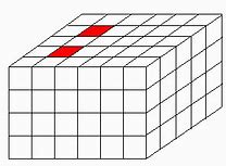
```
   cost_init_volume (the cost cube)
```

The horizontal direction represents image columns, the vertical direction represents image rows, and the inward direction represents the depth (disparity) range. Once the cost volume is built, disparity can be computed even without performing the key cost-aggregation step. Here we skip cost aggregation for now and compute disparity directly from the cost volume.

compute-disparity
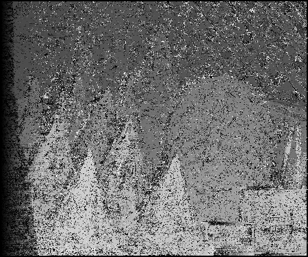
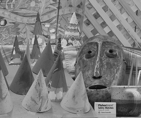
The disparity computation method is very intuitive: for each pixel in the cost volume, we traverse along the disparity direction, and the disparity of the current pixel is chosen according to the principle that the corresponding cost is minimized. After a triple loop, the corresponding disparity map can be generated—this is the so-called WTA (winner take all) principle. After the few simple steps above, we obtain the following result, using the classic left-right sample images from Middlebury College:

Cost Aggregation
Now let’s discuss the most critical cost-aggregation step. This step is the soul of SGM. Let’s first look at the effect:

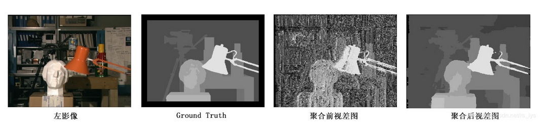
The commonly used cost aggregation schemes are 4-path aggregation and 8-path aggregation. The 4-path aggregation includes top-to-bottom, bottom-to-top, left-to-right, and right-to-left; the 8-path aggregation adds aggregation paths in the 45-degree and 135-degree directions. The purpose of path aggregation is to consider not only local cost information but also global smoothness information. It simply uses one-dimensional aggregations along multiple directions to approximate the two-dimensional problem, achieving similar accuracy with a substantial improvement in efficiency (isn't this a sentence you hear quite often?).

Taking 4-path aggregation as an example, four aggregated cost cubes are obtained separately, and they are summed to obtain the final cost cube:

for(sint32 i =0;i<size;i++) {
    	cost_aggr_[i] = cost_aggr_1_[i] + cost_aggr_2_[i] + cost_aggr_3_[i] + cost_aggr_4_[i];
    	if (option_.num_paths == 8) {
            cost_aggr_[i] += cost_aggr_5_[i] + cost_aggr_6_[i] + cost_aggr_7_[i] + cost_aggr_8_[i];
        }
    }

here size = width * height * disparity_range    

Taking 1-path aggregation in the left-to-right direction as an example, let’s see how to obtain its corresponding cost cube.

The formula for computing an element of the cost cube: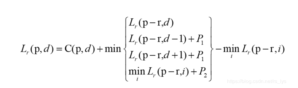

where p represents the pixel position, d represents the disparity value, and r is the traversal path—in the current example, left-to-right—so the current Lr corresponds to cost_aggr_1_ in the code, representing the aggregated cost cube, and C is the initial cost cube. In plain language, the meaning of the formula is:

the value at pixel p, disparity d in the aggregated cost cube = the initial cost value at this position + min(L1, L2, L3, L4) - L4

where:

L1 represents the value at pixel p-r, disparity d in the current cube; in the left-to-right example, this refers to the pixel to the left of the current pixel
L2 represents the cost value at the same left-side pixel but at disparity d-1, plus the p1 penalty term (a small penalty for a disparity change of 1)
L3 represents the cost value at the same left-side pixel at disparity d+1, plus the p1 penalty term (a small penalty for a disparity change of 1)
L4 represents the minimum cost value over all disparity positions (the disparity channel) at the same left-side pixel, plus the p2 penalty term (a larger disparity change corresponds to a somewhat larger penalty)

where

                              p2 = p2_init / (I(p) - I(p-r))

The larger the intensity change, the smaller the corresponding penalty. Why?

At object boundaries, the depth changes greatly, and the corresponding disparity also changes greatly. In this case the penalty should be smaller, so we divide by the intensity change to suppress the penalty term. The aggregated cost designed in this way includes not only the original matching cost but also the disparity variation (the cost of the smoothness term).

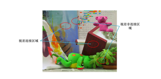
After the operations above, we obtain the final desired aggregated cost cube, and then perform the subsequent optimal disparity computation, etc., based on the cost cube. Having described the entire cost-aggregation process, let’s look at why we do this in theory. Similar to global algorithms, SGM aims to achieve a global optimum, meaning that once the disparity value of each pixel is determined, the overall energy function reaches its optimum:

                                   E(d) = E_data(d) + E_smooth(d)

where the first term is the matching-cost energy, and the second term is the smoothness constraint for surface continuity.

So the core problem is how to solve this two-dimensional optimization problem. SGM does not solve it directly; instead, it uses single-direction aggregation as a one-dimensional approximation, which can also be understood as a form of one-dimensional dynamic programming.

The disparity map formed after only a single left-to-right aggregation pass is as follows:

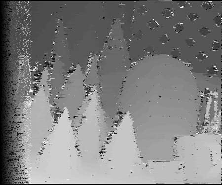
The disparity map after only 4-path aggregation:

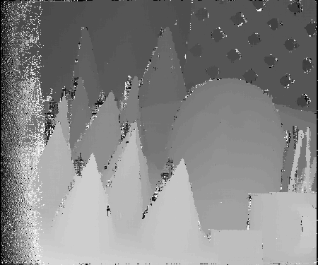
Compared with not performing cost aggregation, we can see the huge effect of this soul step, aggregation. Generally speaking, if efficiency is the goal, 4 paths are sufficient; if better results are desired, 8-path aggregation can be chosen. As can be seen, after aggregation the disparity map already has its basic shape. All subsequent operations refine the aggregated disparity map, and many of the steps in this refinement can be reasonably chosen or omitted according to the actual situation. OK, now we can enter the tedious and detailed disparity-refinement stage.

5 – 8 Disparity Optimization

The purpose of disparity optimization: to improve disparity accuracy, remove erroneous disparities, and make the disparity values accurate and reliable.

Steps 2-4 are all aimed at removing erroneous disparities while maintaining left-right consistency and uniqueness. Adding median filtering of the disparity map can remove disparity noise; bilateral filtering can also be used, which additionally preserves edge accuracy but is slightly less efficient.

The disparity optimization part includes the following sub-modules:

Sub-pixel fitting Fit a parabola through 3 points (x1, y1), (x2, y2), (x3, y3) and find the minimum or maximum (junior-high-school math). After the college entrance exam, my math has regressed to an elementary-school level…
Left-right consistency check

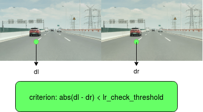
LR check: the disparities of corresponding pixels in the left and right images should be consistent. If the difference between the two is greater than a certain threshold, the disparity of this pixel is set to an invalid value.

dl = Left_Disparity(i,j)
dr = Right_Disparity(i, j - dl)

The graphical meaning of the left-right consistency check is:

The figure below shows the left-right consistency loss in monodepth. Unlike the corresponding-pixel disparity-distance loss in SGM, deep learning methods such as monodepth generate a virtual left image from the right image and the left disparity, and construct a loss in the intensity (appearance) domain against the real left image—similar to the photometric error in the direct method of SLAM.

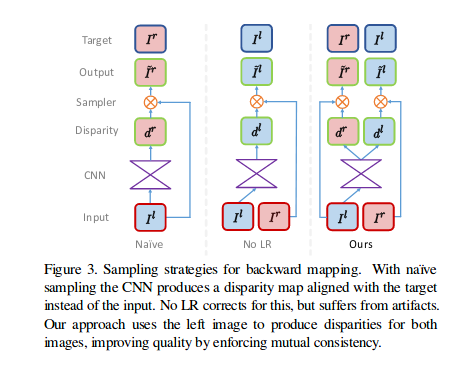
Here comes the question: how is the right disparity map generated? 1) Generate the right-image aggregated cost cube from the left-image aggregated cost cube

             right_cost_aggr[d, h, w] = left_cost_aggr[d, h ,w+d]

2) Generate the right-image disparity map from the right-image aggregated cost cube, as in step 4

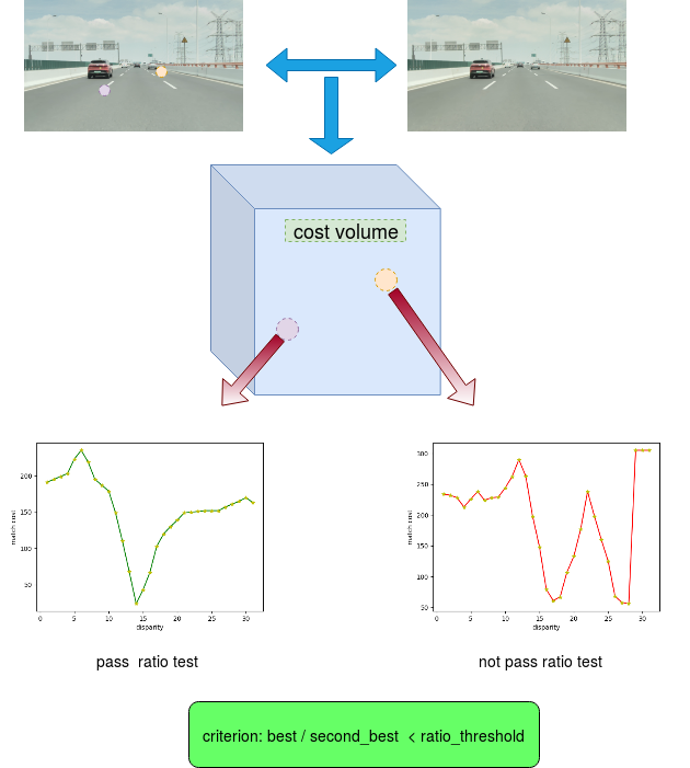
Uniqueness constraint (ratio test) ratio = best_score / second_score If the uniqueness is not sufficiently significant, the current disparity value is set to an invalid value.

note: this is also a robustification strategy commonly used in feature-point matching; its corresponding graphical meaning is:

Small connected-region removal

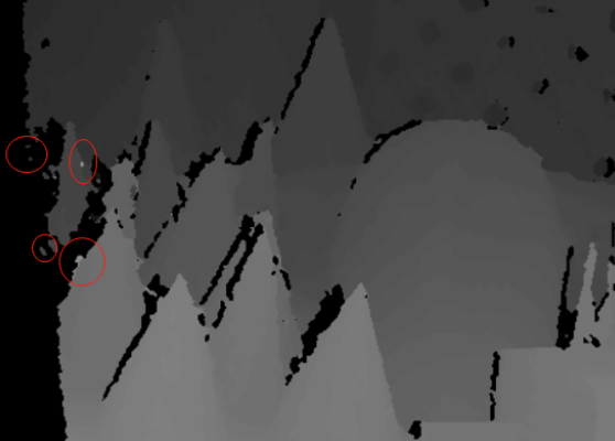
There exist some small connected regions whose disparity is very inconsistent with the overall disparity of the object. Ordinary filtering has difficulty removing such connected regions, so a region-tracking method is used to find regions whose intensity variation lies within a certain range. If the area of such a region is smaller than a certain threshold, the disparities of all pixels within the region are set to invalid values.

method: depth-first traversal to find connected regions (DFS)

Median filtering Remove outlier values (median filter)
Weak-texture region optimization
Hole filling (disparity filling) Whether disparity filling is needed is determined according to the actual requirements. If each pixel is required to be as accurate as possible without requiring completeness, then disparity filling is not needed; if a complete disparity map is required but accuracy is not critical, then disparity filling is needed. Distinguish between occlusion regions and mismatch regions: for occlusion regions, fill with the disparity of background pixels; for mismatch regions, take the median of the surrounding disparities.
- Comparison with learning-based methods such as monodepth
There are 3 loss terms in total. The first is the appearance matching loss:

Photometric error + structural similarity error—this is essentially equivalent to the Hamming-distance matching cost in SGM.

The second term, the Disparity Smooth Loss:

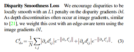
From the formula, we can qualitatively see that the smoothness loss is proportional to the disparity variation and exponentially inversely proportional to the image gradient. The real physical meaning conveyed by the formula is that we do not want large disparity variations in flat regions, yet we also cannot suppress the fact that disparity should change sharply at object boundaries. Isn’t SGM’s soul step, “cost aggregation”, doing exactly this?

The third term, the Left-Right Disparity Consistency Loss:

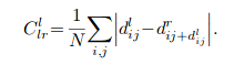
The left-right consistency check from SGM finds its application in monodepth.

After looking at the comparison of the several technical points above, doesn’t it seem that the so-called monodepth is merely a subset of the SGM technique set? In the context of deep learning, the ideas from SGM are wrapped in various ways so that they can run under the learning paradigm, thereby estimating depth in the form of a huge number of parameters. Leveraging the powerful expressive capability of deep learning, the accuracy of disparity estimation is significantly improved. However, it cannot be denied that deep learning methods may suffer from some generalization issues.

tight fusion at the loss level

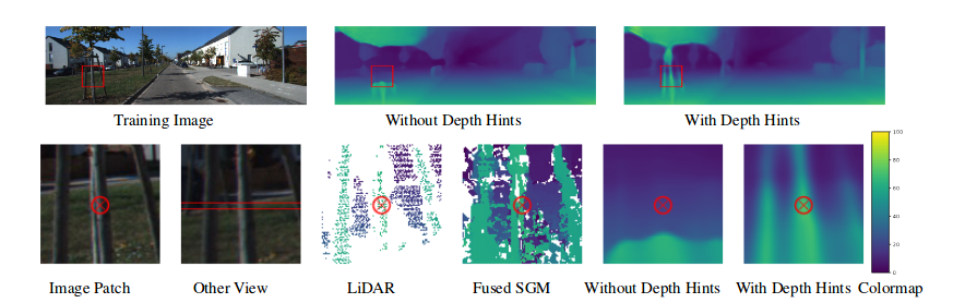
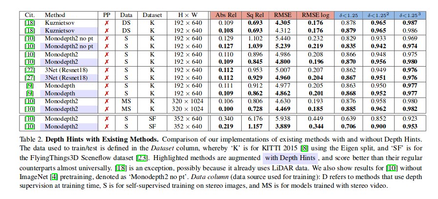
At the same time, monodepth leaves many ideas from SGM unwrapped—is there room for further development? We can also see that nianticlabs (https://github.com/nianticlabs), the organization that released monodepth2, also released a new improved version last year, depth hints (https://arxiv.org/pdf/1909.09051.pdf), which achieves better depth estimation results by fusing SGM supervision information during training:

The above is my brief personal summary of stereo matching. If it helps your work or research, it would be my greatest honor. If you have any questions, feel free to contact me.

cell phone: 13162517010
email: candyguo_fly@163.com

If you find this blog helpful, please consider sponsoring me, so that I can be more motivated to keep updating the blog.

Stereo Matching

Stereo Matching

Stereo Matching

SGM

Comments