Paper Reading Part2

LVI-SAM: Tightly-coupled Lidar-Visual-Inertial Odometry via Smoothing and Mapping (ICRA 2021)

• lvi-sam Tightly-coupled lidar-visual-inertial odometry: LVI-SAM builds a factor graph composed of two subsystems, LIS and VIS. Both subsystems are designed in a tightly-coupled manner, and LIS and VIS can reinforce each other. Initialization of VIS is relatively difficult and requires a certain amount of accelerated-motion excitation; VIS can leverage the estimates from LIS to complete its initialization. Meanwhile, depth estimation of visual features is a fundamental component in visual SLAM, and the visual features of VIS can obtain depth information from lidar measurements, thereby improving the accuracy of VIS. When LIS performs scan-matching-based pose estimation, it can use the VIS estimate as an initial value. In the loop-closure part, loop closures can be confirmed by VIS using visual appearance information and then further optimized by LIS. Because these two subsystems reinforce each other, LVI-SAM can still operate when one of them fails, such as when texture is missing (where VIS tends to fail) or geometric features are missing (where LIS tends to fail).

vins + liosam

• Introduction: Over the past 20 years, single-sensor-based SLAM technology has developed rapidly, including camera-based SLAM, lidar-based SLAM, and radar-based SLAM. Each has significant advantages and disadvantages. Starting five or six years ago, VI systems and LI systems received a great deal of attention and research. Combining a single visual sensor or lidar with a cheap inertial measurement unit significantly improves their respective accuracy and robustness. For LI systems, the IMU can help correct point-cloud distortion during motion and address the problem of short-term feature loss. For VI systems, fast motion, scale recovery, and the provision of initial values for state estimation can all be obtained from IMU information. This paper combines two currently widely used works, VINS-Mono and LIO-SAM, and proposes a tightly-coupled LVI-SAM framework via smoothing and mapping. The VIS in LIO-SAM performs visual feature tracking and selectively uses lidar frames to obtain feature depth. The VIO obtained by optimizing the visual reprojection error and the IMU measurement error can serve as the initial value for scan matching in the LIS system. After correcting the point cloud using IMU information, LIS extracts edge and planar point-cloud features and matches them against the feature map in the sliding window. The state estimated by LIS can be sent to VIS to facilitate its initialization. Constraints from VO, LO, IMU pre-integration, and loop closure are jointly optimized in the factor graph. The optimized IMU bias is used to propagate the IMU measurements, enabling state estimation at the IMU rate. LVIO represents a unique integration of the state of the art in VIO and LIO.

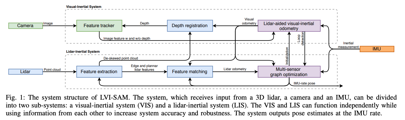System architecture of LVI-SAM. VIS and LIS can run independently of each other, or leverage each other’s information to improve accuracy and robustness. The system ultimately outputs poses at the IMU frequency.

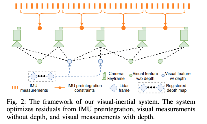Flowchart of the visual-inertial system.

GFTT is used for feature extraction and KLT for feature tracking between frames. Compared with the original VINS, the initialization and feature depth estimation parts are improved.

• Initialization Initialization of the VIS system is relatively difficult, and its quality depends on two factors: the initial motion of the sensor and the accuracy of the IMU parameters. When the VINS sensor moves at a low or constant velocity, initialization usually cannot be completed, because scale is unobservable when there is insufficient acceleration excitation. The IMU parameters include slowly time-varying bias and white noise, which affect both the raw acceleration and angular velocity measurements; having a good estimate of these parameters at initialization time is beneficial for the convergence of the nonlinear optimization problem. The state estimate from LIS is used to help VIS complete initialization: because lidar depth is observable, the lidar measurements can be used directly to estimate the system state and the IMU bias. The states are then interpolated according to the estimated states and the image timestamps and associated with image keyframes. Finally, the interpolated image states and IMU bias are used as the initial values for VIS initialization, which significantly improves the speed and robustness of initialization. vis init video

• Feature depth association

To associate feature points with depth values, visual features and lidar depth points are projected onto a unit sphere centered at the camera. Multiple frames of the lidar point cloud (a single frame is too sparse) are projected into the camera coordinate frame using the camera-lidar extrinsics and then onto the normalized sphere via the imaging model. The depth points are downsampled and stored using polar coordinates. A two-dimensional KD-tree is searched using the polar coordinates of the visual feature to find the three nearest depth points on the sphere. Finally, the bearing vector of the feature intersects the plane formed by the three depth points in Cartesian space, as shown in the figure: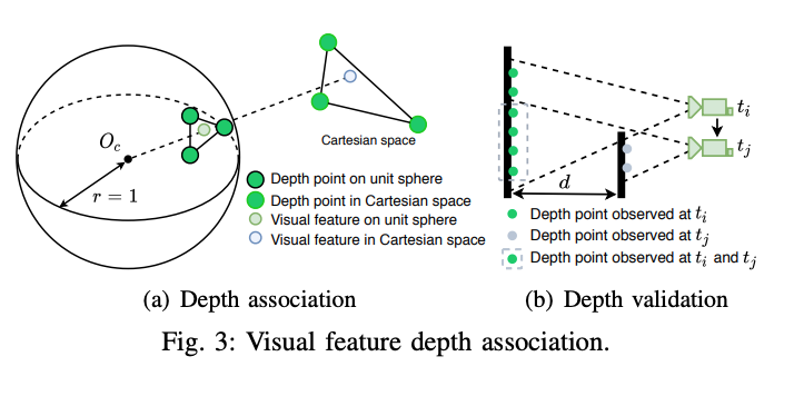

Validity is further determined by checking the depth differences among the three points.

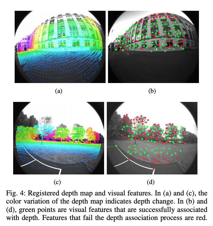
The figure above shows the registered depth map and visual features. Green points are features successfully associated with depth, and red points are features for which depth association failed.

• Failure detection VIS tends to fail under aggressive motion, illumination changes, and in texture-less areas. Therefore, when the number of tracked features falls below a threshold, or when the estimated IMU bias exceeds a threshold, a VIS failure is reported, VIS is re-initialized, and LIS is notified.

• Loop-closure detection DBoW is used for loop-closure detection. The timestamps of the candidate loop-closure images returned by DBoW are sent to LIS for further verification.

LIS system:

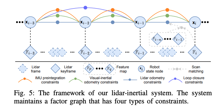
The entire factor graph contains four types of constraints: IMU pre-integration constraints between keyframes, visual odometry constraints, lidar odometry constraints, and loop-closure constraints. The lidar odometry constraints come from scan matching, which matches the current lidar keyframe against the global point-cloud feature map. The candidate frames for loop-closure constraints are first provided by VIS and then further optimized through scan matching. A sliding window of lidar keyframes is maintained for the lidar point-cloud local map; when the platform moves beyond a certain threshold, a new keyframe is created, and after a new lidar keyframe is selected, the new platform state is added as a node to the factor graph. Two aspects that improve system robustness:

1. LIS initialization After LIS initialization, the initial estimate is obtained from two sources: one is the integration of bias-corrected IMU measurements, and the other is VIS. When VIS information is available, VIS is used as the initial estimate for scan matching; if VIS fails, the system switches to IMU measurements for initialization.
2. Failure detection To judge the validity of scan matching, the smallest eigenvalue of A^T * A is computed; when it is below a certain threshold, LIS is deemed to have failed. When a failure occurs, the lidar odometry constraint is not added to the factor graph.

$ min(||AT - b||) $ A least-squares problem that scan matching aims to solve.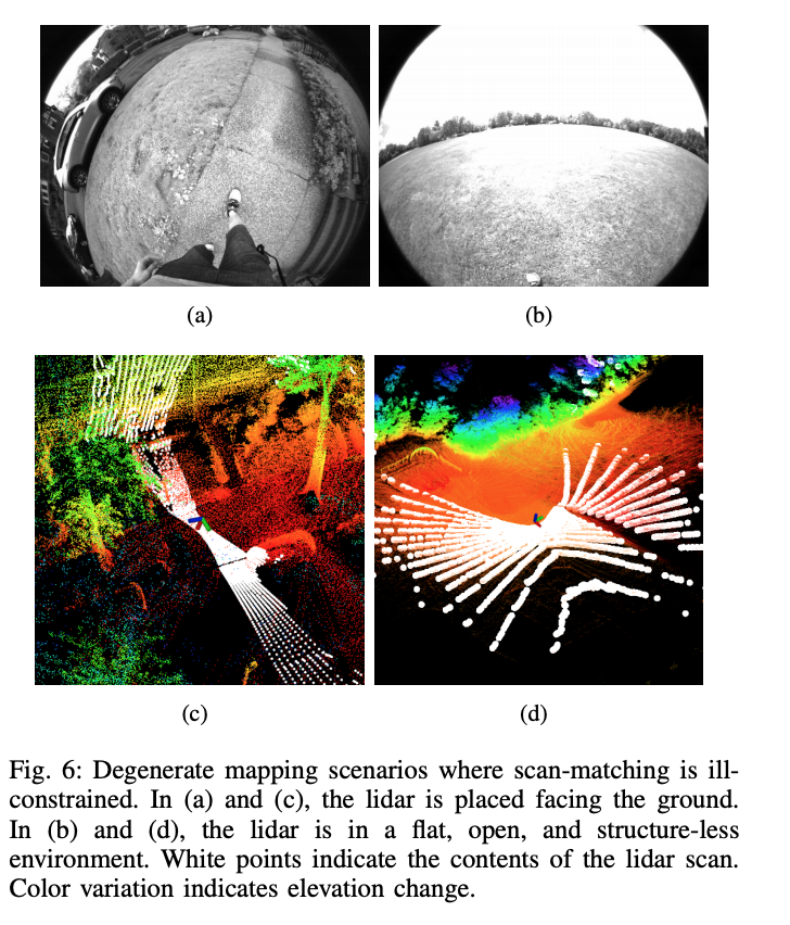

In open areas, or when the lidar observes downward, scan matching degenerates and is prone to matching failure.

Ablation study

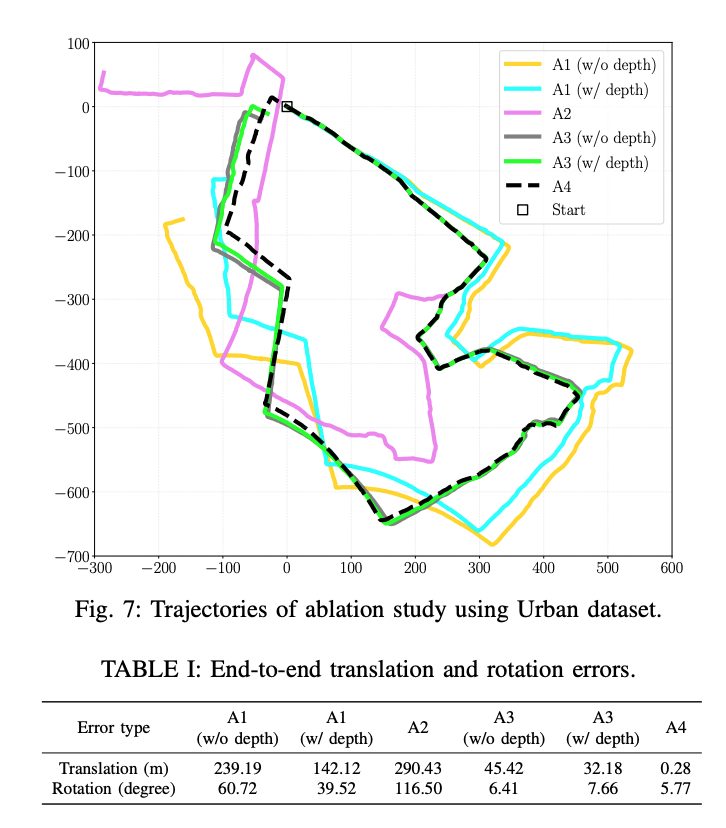
A1: The effect of lidar feature-point depth on VIS. Scan matching in LIS is disabled and only VIS is relied upon for pose estimation. It can be seen that, compared with not using depth cues from the lidar point cloud, using lidar points to provide feature depth effectively improves accuracy.

A2: VIS is disabled and only LIS is used for pose estimation. It can be seen that performance is poor when encountering degenerate scenes.

A3: LIS and VIS are used together, with the depth registration module switched on. It can be seen that the pose error is greatly reduced.

A4: Loop-closure detection is enabled, eliminating accumulated drift.

• Jackal dataset

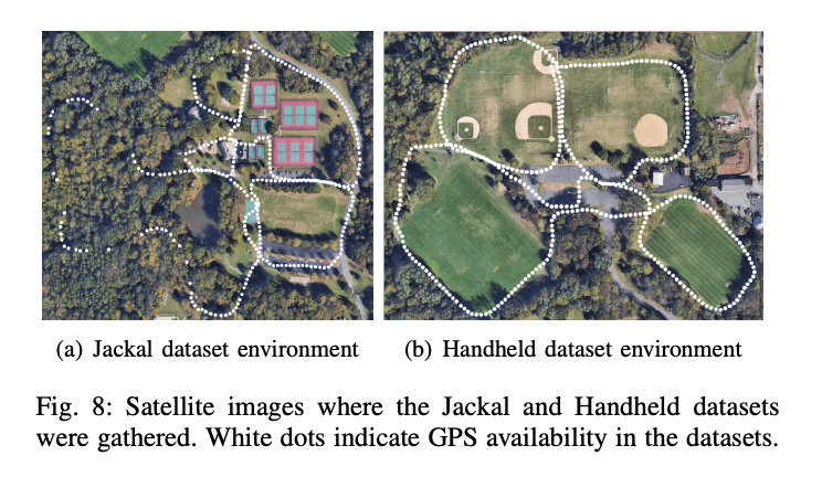
• Handheld dataset

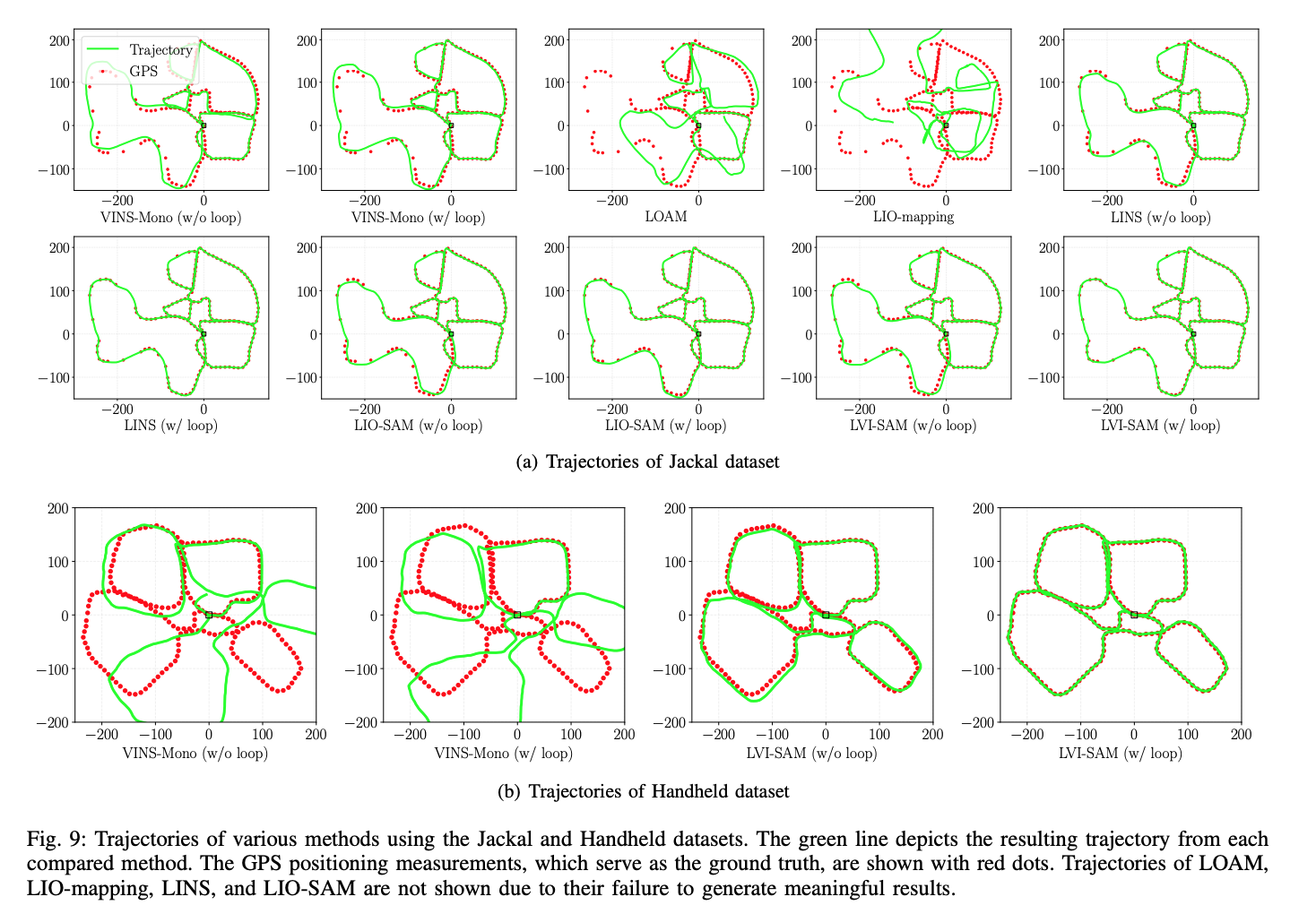
With added sensors, the results are naturally improved:

Accuracy evaluation: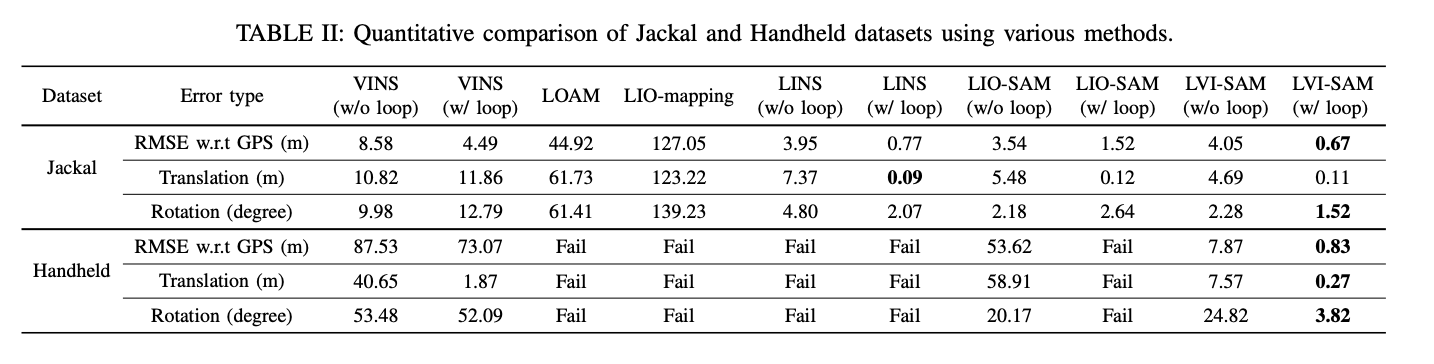

Generalizing to the Open World: Deep Visual Odometry with Online Adaptation

Deep-learning visual odometry with online adaptation

Classical SLAM/VO algorithms rely on low-level features as the image representation and perform poorly in weakly-textured, dynamic environments. Deep neural networks can extract high-level features and be optimized end-to-end through learning. Among these algorithms, self-supervised VO algorithms can jointly learn camera pose, depth, and optical flow by minimizing the photometric error. However, pre-trained networks perform poorly when facing different scenes, so pre-trained networks need to achieve online adaptation in a self-supervised manner.

The overall architecture is shown in the figure below: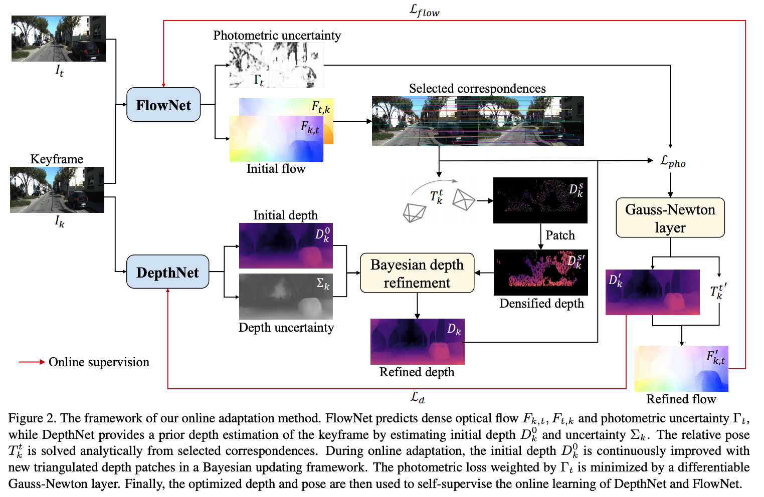

OV2SLAM : A Fully Online and Versatile Visual SLAM for Real-Time Applications

Orthographic feature transform for monocular 3D object detection

The ability to reason about the 3D world is a fundamental element of the 3D object detection task. This work introduces the orthographic feature transform, which escapes the image domain by mapping image-based features into an orthogonal 3D space. This enables holistic reasoning about the spatial configuration of the scene in a domain where scale is consistent and inter-object distances are meaningful. This paper applies this transform as part of an end-to-end deep-learning architecture.

In the perspective projection of an image, the scale of an individual object varies considerably with the object’s distance from the camera, its appearance changes greatly as the viewpoint changes, and 3D distances cannot be inferred directly. A commonly used representation is the bird’s-eye view, for example in lidar-based perception, in which scale is uniform and appearance is independent of viewpoint. The authors argue that reasoning should be performed in this view as much as possible, rather than in the original image domain. Based on this, the authors propose OFT, a differentiable orthographic transform that can map a set of features extracted from the perspective view into an orthographic bird’s-eye view.

Overall architecture: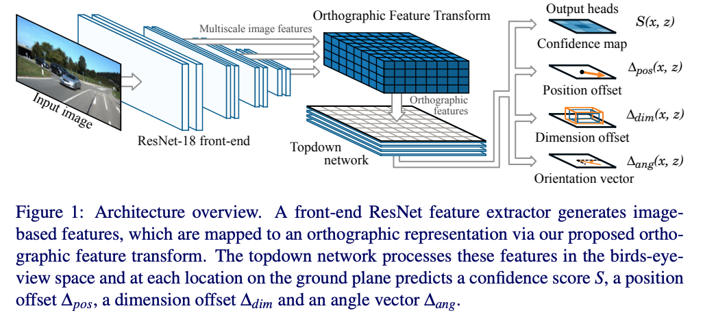

The algorithm consists of five parts:

1. An initial ResNet feature extractor performs multi-scale feature extraction on the original image.
2. OFT, which converts the image-based features at each scale into an orthographic bird’s-eye-view representation.
3. A top-down network composed of a series of ResNet residual units, which processes the feature map from OFT.
4. A set of output heads that predict a confidence score, position offset, dimension offset, and orientation vector at each location on the ground plane.
5. An NMS & decode stage that identifies peaks and generates discrete bounding-box predictions.

oft part detail:

The goal of OFT is to populate a 3D voxel feature map with the relevant n-dimensional features from the feature map extracted by the front-end feature extractor. The voxel feature map is defined on a uniformly spaced 3D grid at a fixed distance from the ground plane, with dimensions W, H, D and voxel size r, as shown in the figure below: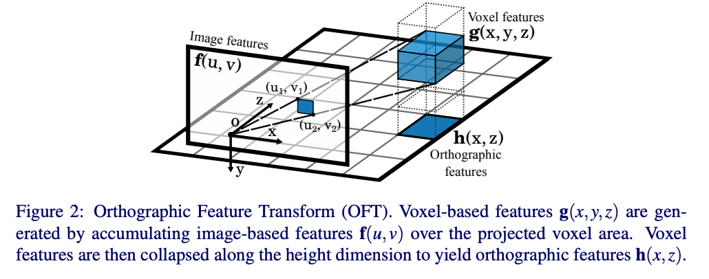

The region corresponding to a voxel is mapped onto the image, and the mapped polygon is approximated by a rectangular box whose coordinates are computed using the following formula:

Average pooling is performed over the values within the projected region to obtain the value of g(x, y, z), as shown in the following equation:

The resulting voxel feature map is already a scene representation that is unaffected by perspective; however, running a deep neural network on such a 3D voxel grid is very memory-intensive. Since most objects in autonomous driving lie on the ground plane, the voxel map is collapsed into a 2D representation called the orthographic feature map h(x, z).

The orthographic feature map is obtained by multiplying the voxel feature map by a learned weight matrix and summing along the vertical axis.

• Fast average pooling using integral images

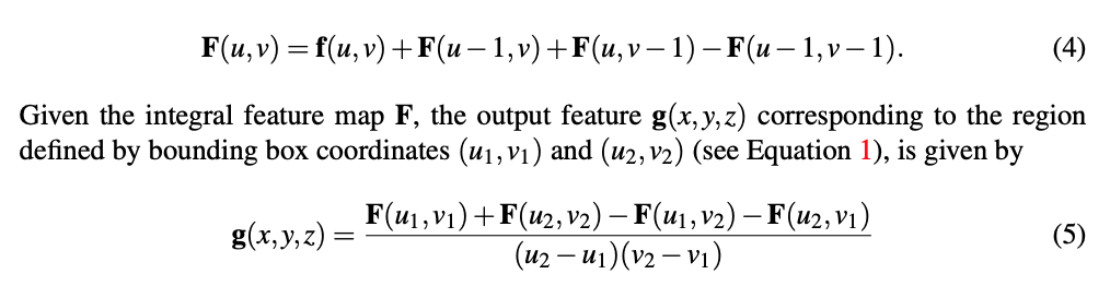
top-down network part detail: The top-down network is a simple convolutional network that uses ResNet-style skip connections and is applied to the 2D feature map generated by the OFT stage.

• head output Confidence map prediction: The confidence map is a smooth function representing the probability that an object with a bounding box centered at position (x, y0, z) exists at that location. So how is the GT confidence map generated? Given the ground-truth bounding-box centers pi = [xi, yi, zi] of N ground-truth objects, the ground-truth confidence map is computed as a smooth Gaussian region, as shown in the following equation:

The confidence map is trained with an L1 regression loss. Since the number of positive samples is far smaller than that of negative samples, a constant factor of 0.01 is introduced and multiplied onto the negative-sample locations (S(x, z) < 0.05) to reduce the influence of the large number of negative samples.

Object position and bounding-box estimation: An additional head is added to predict the relative offset of the object center position, as shown in the following equation:

Two additional heads predict the dimensions and orientation.

The position offset, dimension offset, and orientation vector of each cell are trained with an L1 loss, ignoring cells that do not contain any object.

• NMS NMS is used to obtain the final discrete object predictions. Unlike the bounding-box overlap computation in conventional 2D object detection, here the confidence map is smoothed to find peak locations, excluding peak values below a certain threshold.

Experiments: Network architecture: The front-end feature extractor uses a ResNet-18 without bottleneck layers, extracting features before the last three downsampling layers to obtain a set of feature maps at scales of 1/8, 1/16, and 1/32 of the original input resolution. A 11 convolution kernel converts the feature maps to a specific size of 256, and then OFT produces the orthographic feature map h. The voxel grid size used in the paper is 80m4m80m with a grid resolution of 0.5m. The top-down network uses a simple 16-layer ResNet without downsampling or bottleneck layers, and each output head consists of a single 11 convolution. GN is used instead of BN, since GN performs better on small-batch data.

Dataset: kitti 3d object detection benchmark, training dataset: 3712, validation dataset: 3769

data augmentation: random crop, scaling, horian flip

training procedure: SGD is used, 600 epochs, batch size: 8, momentum: 0.9, learning rate: 1e-7

Performance on the KITTI benchmark: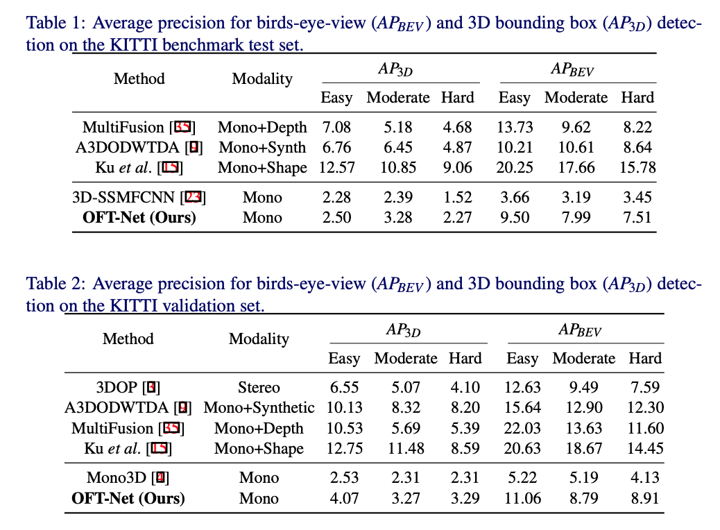

Qualitative evaluation:

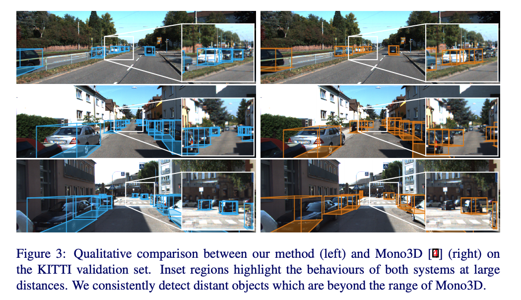
From the figure, it can be seen that the performance at longer ranges is somewhat better.

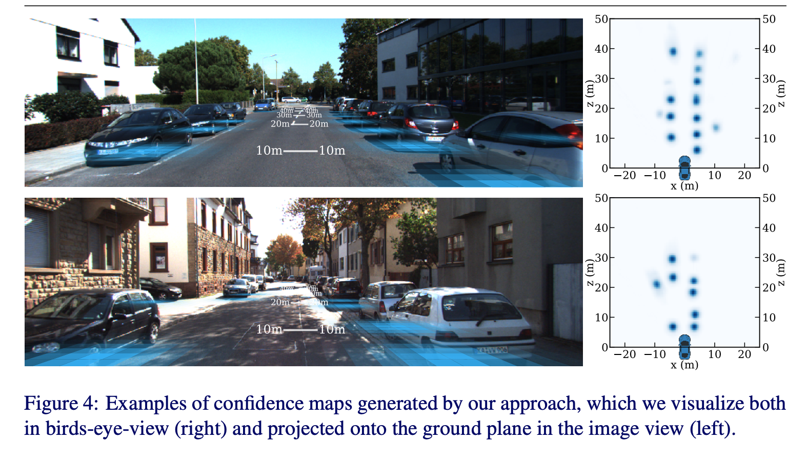
The confidence map in BEV and its projection onto the original image.

ablation study: The ablation study verifies the role of the top-down network.

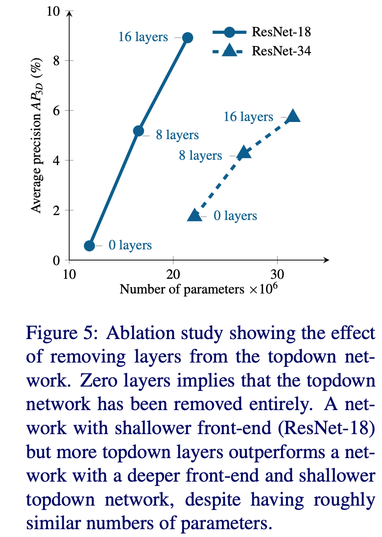
A shallow feature-extraction network + a deep top-down network works better.

The figure shows the evolution of the confidence map during network training. At the beginning, the network can quickly locate the approximate region of an object, but with high uncertainty. As training progresses, the localization uncertainty decreases, but distant objects still exhibit uncertainty, demonstrating the difficulty of localizing distant objects.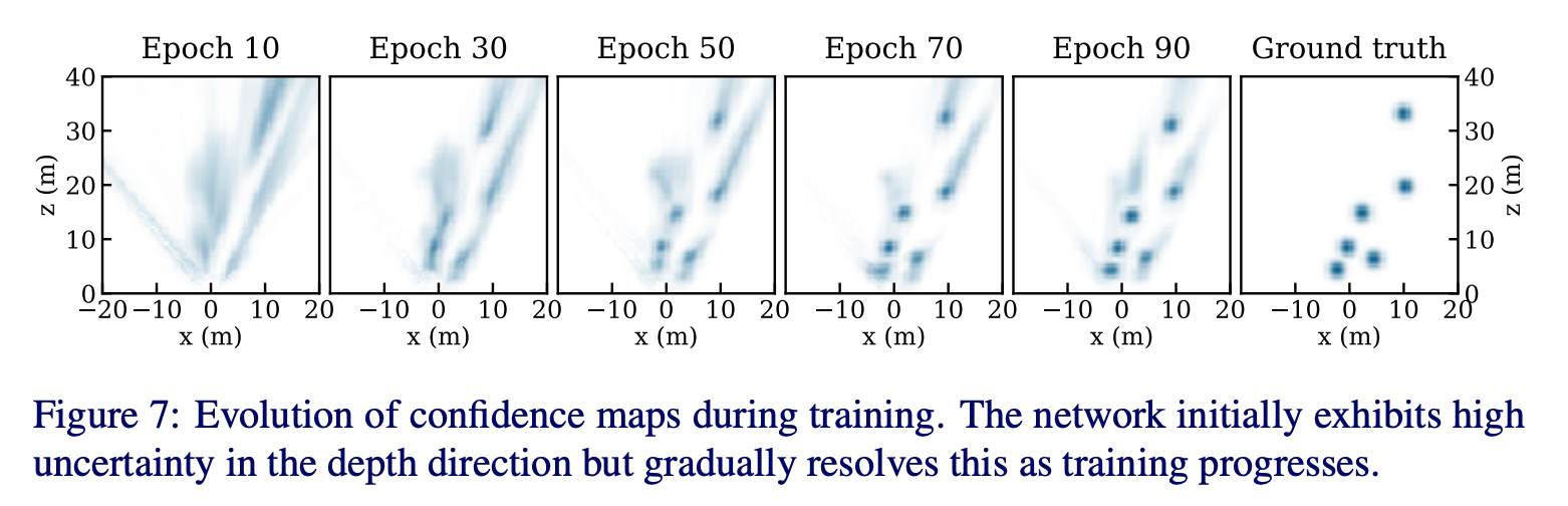

RoadMap: A Light-Weight Semantic Map for Visual Localization towards Autonomous Driving

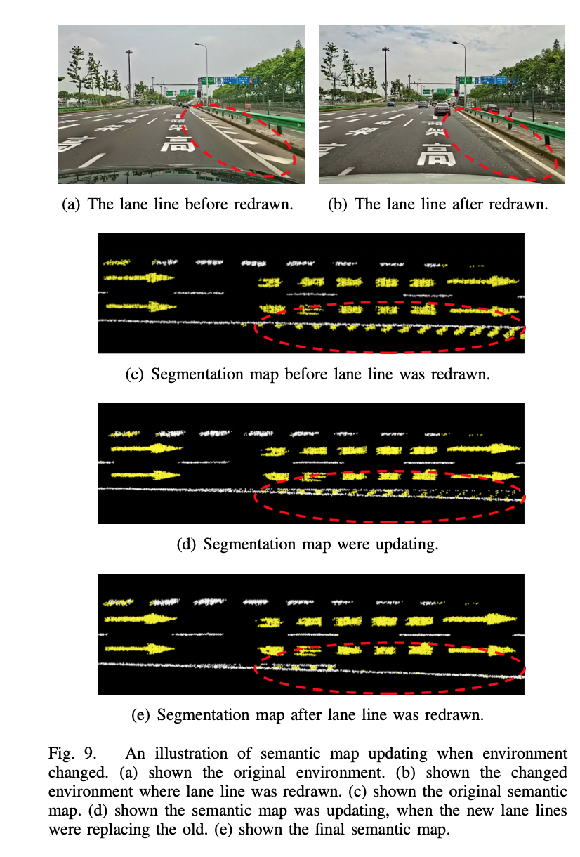
The paper proposes using sensor-rich vehicles for on-vehicle crowdsourced mapping. The crowdsourced local maps are aggregated in the cloud, the aggregated global map is compressed in the cloud, and the compressed map is transmitted to the vehicle and decompressed, finally using on-vehicle perception for localization. (Of course, if low-cost on-vehicle localization is eventually accurate enough, low-cost vehicles can also be used for crowdsourced map updates.) So a sensible pipeline is as follows: use maps from third-party map providers or crowdsourcing from robotaxi vehicles to form a base map, then maintain it in the cloud and perform map fusion, and finally perform map updates while localizing on consumer-grade vehicles.

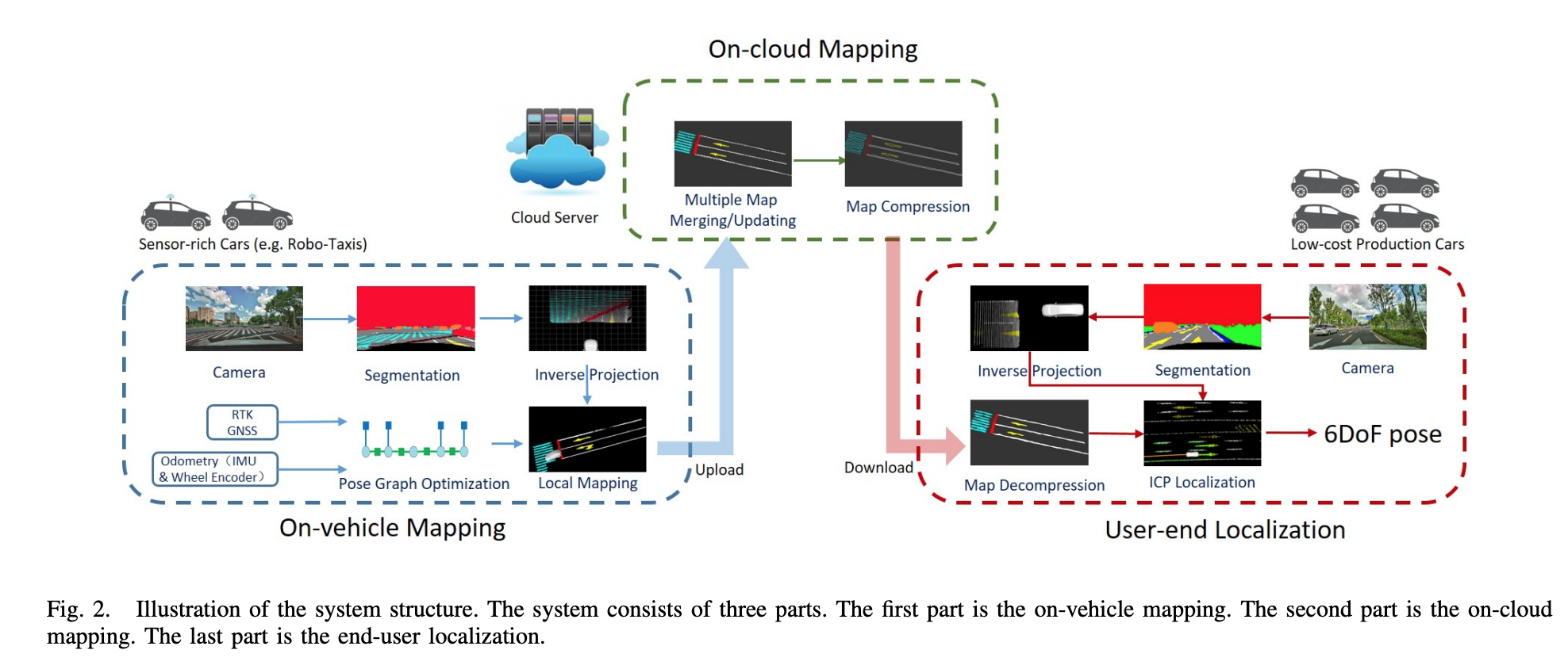
vehilce mapping

First, semantic segmentation is performed on the original image. Then the segmented pixels are projected into the vehicle coordinate frame using the camera’s intrinsics and extrinsics relative to the vehicle. Because of the noise in image segmentation, only the ROI region inside the red box is back-projected.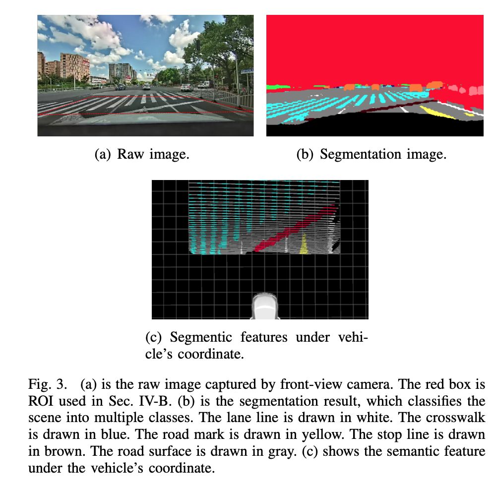

Because mapping requires accurate poses, and RTK-GNSS already provides centimeter-level localization in unoccluded areas, pose-graph optimization is used to average out pose errors and obtain continuous, consistent poses, so that occluded areas also achieve high localization accuracy.

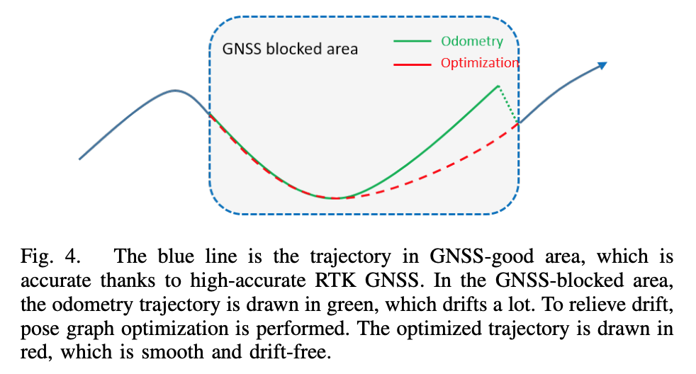
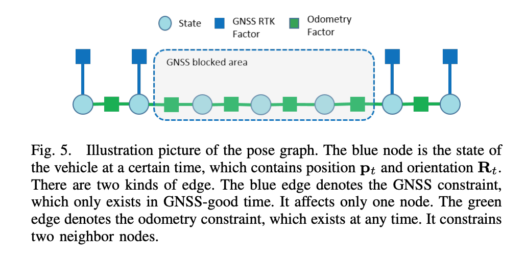
Because of segmentation noise, observations from multiple frames are used to determine the class corresponding to a given map location. The map is divided into grids of 0.1 * 0.1 * 0.1, and each grid cell contains a position, a semantic label, and the count of each semantic label. When a semantic point of the corresponding class is inserted into a grid, the count of the corresponding label of that grid is incremented by 1. Finally, a max-voting, winner-takes-all scheme is used to decide the grid’s class.

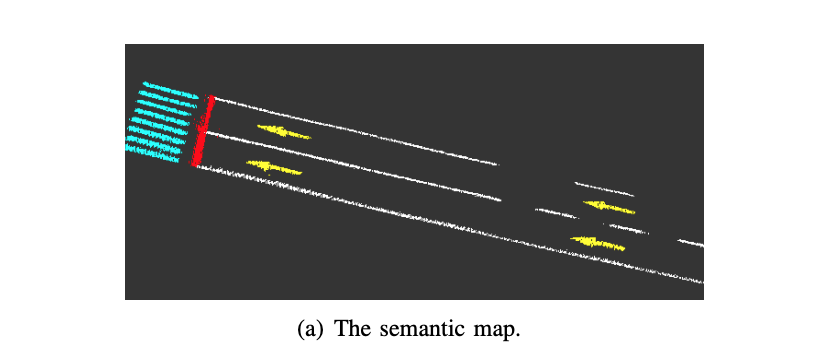
cloud mapping

The cloud is responsible for aggregating the local maps built by vehicles over multiple drives. To save bandwidth, only occupied grids are uploaded. The semantic map in the cloud is also divided into grids, and the grid scores of the local maps are added to the corresponding grids of the global map.

To further save bandwidth, the map transmitted to the vehicle is compressed, reducing the map size through contour extraction.

user vehicle localization

During localization, the current map points in the perceived vehicle coordinate frame are registered against the map points in the semantic map via ICP to estimate the current vehicle pose. An EKF is introduced to couple the odometry observations and output a smooth trajectory.

Progressive results of the map update: