Vision Global Localization With Semantic Segmentation And Interest Feature Points (IROS 2020)
Paper Analysis
Vision Global Localization with Semantic Segmentation and Interest Feature Points (IROS 2020)
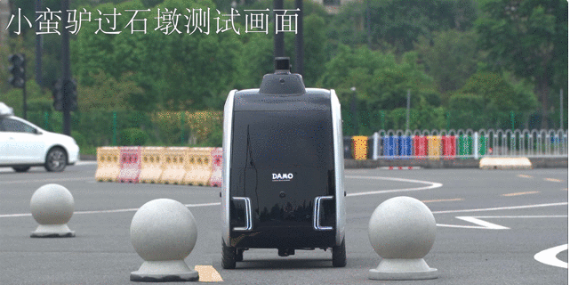
The authors are from Alibaba and OPPO. The localization algorithm described here has been deployed on Alibaba’s logistics autonomous delivery vehicles.
INTRODUCTION
Visual global localization is mainly divided into two categories:
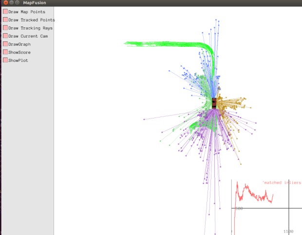
Nonlinear optimization based on tracking & matching using a global map (e.g. the localization mode in ORB-SLAM2)
End-to-end learning networks for place recognition (PoseNet, HF-Net, etc.)
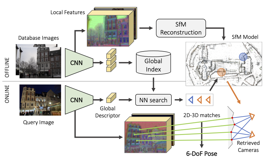
- hfloc diagram -
As a traditional approach, structure-based visual localization methods can also be divided into two categories:
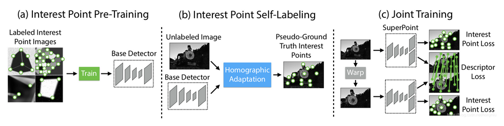
Matching the features extracted from the current frame against a pre-built map. This relies heavily on the repeatability and consistency of features under different conditions; deep-learning features, represented by SuperPoint, have demonstrated better robustness and performance.
Using semantic segmentation features as cues for localization estimation. These features are relatively robust, but not everywhere has rich semantic information, which limits the applicable scenarios.
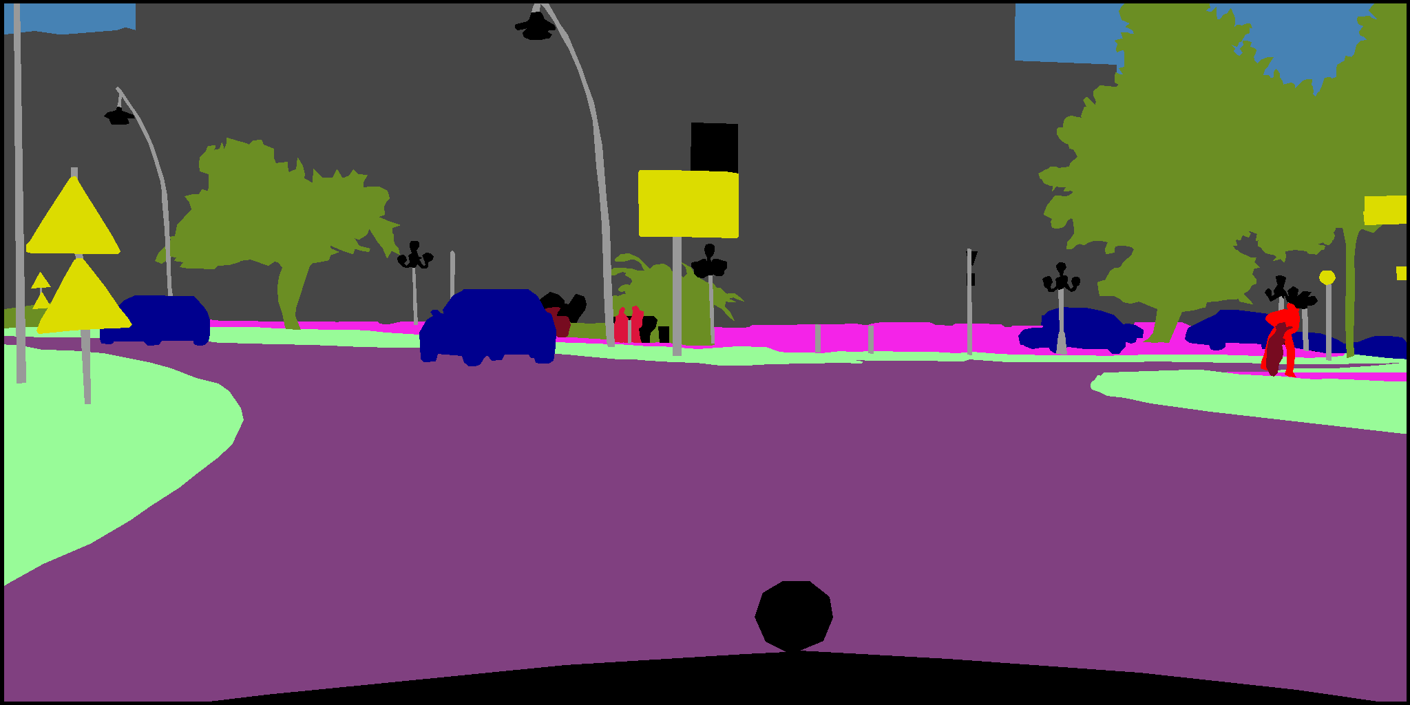
Considering the robustness of semantic segmentation features and the ubiquity of interest feature points, the constraints from both types of features are used simultaneously during state estimation to achieve robust, high-precision localization.
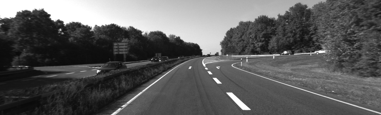
- Abundant semantic features, sparse feature-point features -
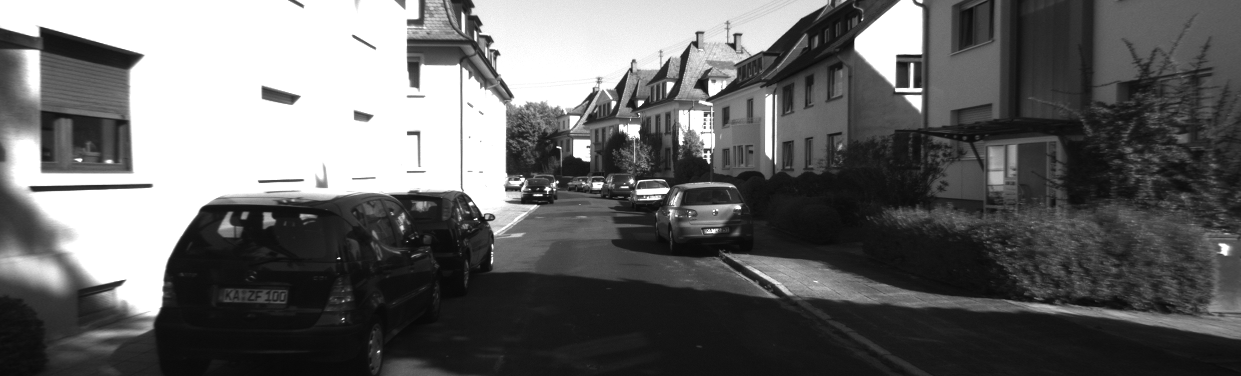
- Missing semantic features, rich feature-point features -
METHOD OVERVIEW
First, pixel-wise semantic segmentation is applied to the front-facing monocular image to extract semantic features, such as:
pole-like objects
lane-markings
curb
These high-level features are robust to illumination changes and viewpoint changes. Considering that the semantic features in many places are not rich,
interest feature points are then extracted on the static scene, and the semantic segmentation mask can also be used to filter them.
Since both types of features are used simultaneously, two map layers need to be built:
- The semantic map layer, built from a LiDAR point cloud semantic map,
- The feature-point map layer, built through a fixed-pose SFM process. This fixed pose can come from a high-precision INS system, or from a 3D LiDAR SLAM system, which is more accurate than vision.
Finally, the residuals formed by the observations of both types of features are combined, and the LM optimization algorithm is used to solve for the pose that minimizes the cost.
PIPELINE
The overall pipeline diagram is as follows: 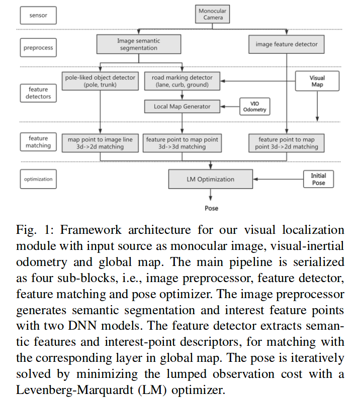
Two deep-learning models perform feature-point extraction and semantic segmentation respectively; then different matching and residual construction are performed for the different features, and finally the pose is solved through optimization.
IMAGE PRE-PROCESS
Because the processor used is resource-constrained, the network needs to be efficient while maintaining a high mIoU. BiSeNet was chosen for the segmentation network, and SuperPoint was chosen for feature-point detection and description.
BiSeNet Speed-accuracy diagram:
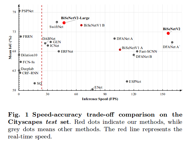
The original BiSeNet network architecture diagram is as follows: 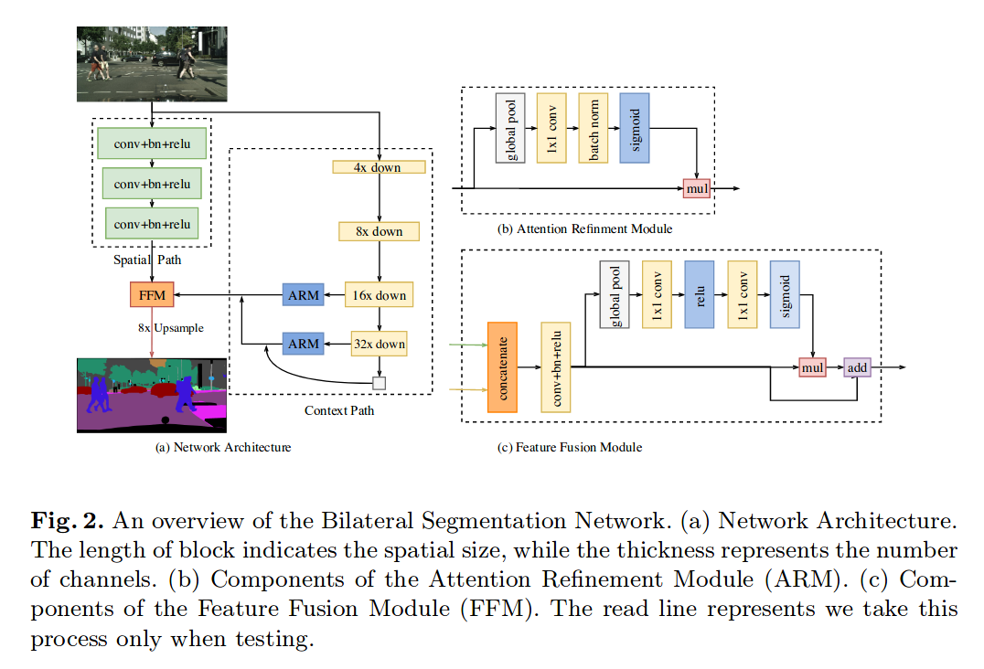
As you can see, it contains two paths:
spatial path
The spatial path is a combination of three conv + bn + relu blocks, each convolution having a stride of 2, ultimately outputting a feature map at 1/8 of the original image resolution. The spatial path encodes rich spatial information.
context path
The context path provides a sufficient receptive field (in semantic segmentation, the receptive field has an important impact on the final performance), using a lightweight model to down-sample, followed by an ARM module that passes to the FFM for the final feature fusion. Within the ARM module, global average pooling is used to capture global information, and an attention vector is computed to guide feature learning.
The two paths run in parallel: the spatial path yields detailed low-level information, while the context path encodes high-level contextual information; they enter the FFM module via concatenation.
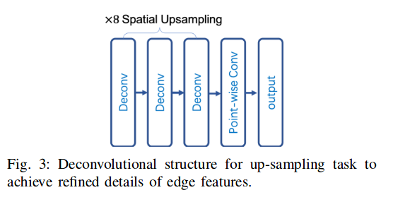
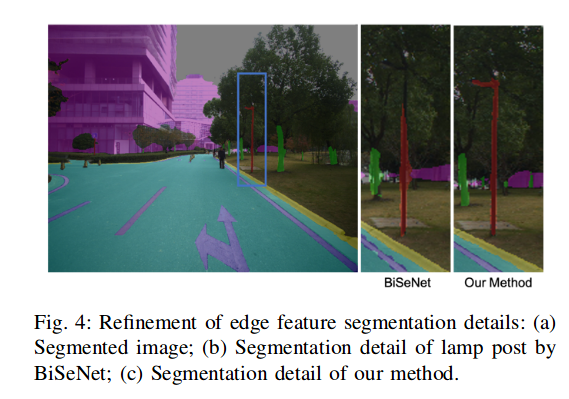
However, BiSeNet performs poorly when segmenting pole-like objects; by improving the upsampling step, a better result is achieved:
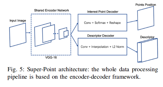
The structure of the SuperPoint feature-point extraction network is as follows:
VISION FEATUR EXTRACTION
- For the extraction of ground features, as shown in the figure:
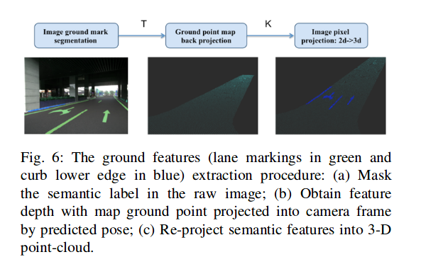
The semantic feature points are back-projected to 3D according to their depth values, forming a 3D-3D matching residual. The depth values are recovered by searching for the projections of nearby mark points in the map, taking the depth of the nearby projected points as the depth of the marker point. After the depth is recovered, the points are back-projected to 3D according to the depth.
ground sampled features
The extraction process is similar to that of lane markings.
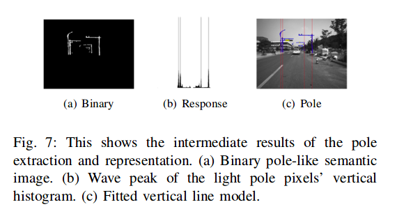
Extraction of pole-like features
- Convert the segmentation result of the poles into a binary image, and fill holes through morphological operations
- Compute a histogram over the columns
- Least-squares fitting
- Interest feature point
Select the feature points that can be stably tracked across multiple frames, and remove the feature points on dynamic objects.
Construction of the Global Map
Semantic feature map (a feature map with semantic labels)
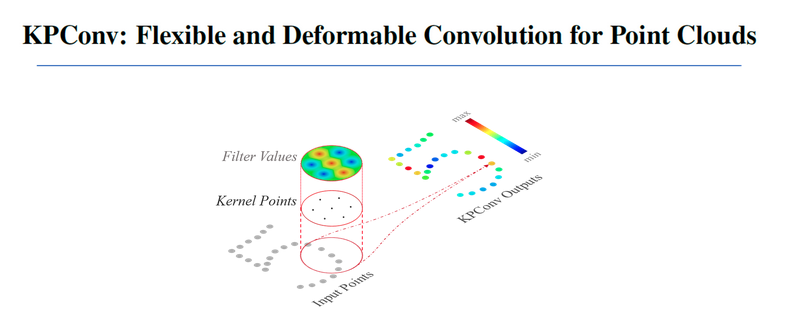
First, a high-precision point cloud map is built from the INS system and multiple 3D LiDARs; then a DNN model on the point cloud (KPConv) is used for classification, yielding a semantic-level point cloud.
KPConv (kernel point convolution) (https://github/HuguesTHOMAS/KPConv) is a convolution method on point clouds that can be used for point cloud segmentation and classification.
The lane-marking points and curb points can be obtained directly from the network output.
As for the processing of ground points, since ground points are important for depth estimation during reprojection, further processing is performed:
- Denoise the ground points
- hole filling
Based on the MLS (moving least squares) method.
- Construction method for the 3D pole map: a. Euclidean clustering of the point cloud to obtain instance-level pole-like object points b. RANSAC fitting of a seven-parameter cylindrical model for the pole-like object c. Merge multiple poles that are broken apart in the vertical direction d. Store the pole endpoints and cylindrical parameters in the map
- For the Feature Point Map: Fixed-Pose SFM, aligning the two maps.
COLMAP (https://github.com/colmap/colmap) is used to build the feature-point map, with the pose coming from the LiDAR SLAM backend.
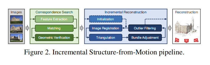
Since visual features are not robust to illumination, there are errors during reprojection and feature matching, making the reconstruction inferior to LiDAR mapping. With the aid of the LiDAR point cloud, a kd-tree nearest-neighbor search is used to remove some outlier points from the visual map.
Optimization
ground marker feature The ground markers from multiple frames are aggregated to form a local map; a kd-tree search over the global map forms 3D-3D correspondences, thereby forming the matching residual.
ground sampled point The residual is the distance from the sampled ground points to the plane.
pole-like object Match the poles projected from the map with the poles in the image, using the distance from the map-projected points to the line in the image as the residual. The pole in the map is described by three points, and the residual is the sum of the distances from these three points to the line.
interest point feature The point features in the map are projected onto the image according to the predicted pose, then matched by descriptor distance. RANSAC is performed to remove mismatches, and finally the inlier matches are added to the final cost term to construct the reprojection error.
- solver:
huber loss function, different weights for different types of features, stack residuals and Jacobians, and the Ceres solver performs the nonlinear optimization.
Experimental Results
- Hardware configuration:
Autonomous delivery vehicle
Hikrobot industrial image sensor (1280 * 1024, 10 Hz)
low cost mems imu
wheel encoder (2,3,4 for vio running)
Intel 8700 CPU, NVIDIA 2080 GPU
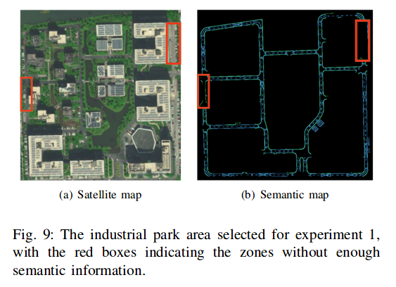
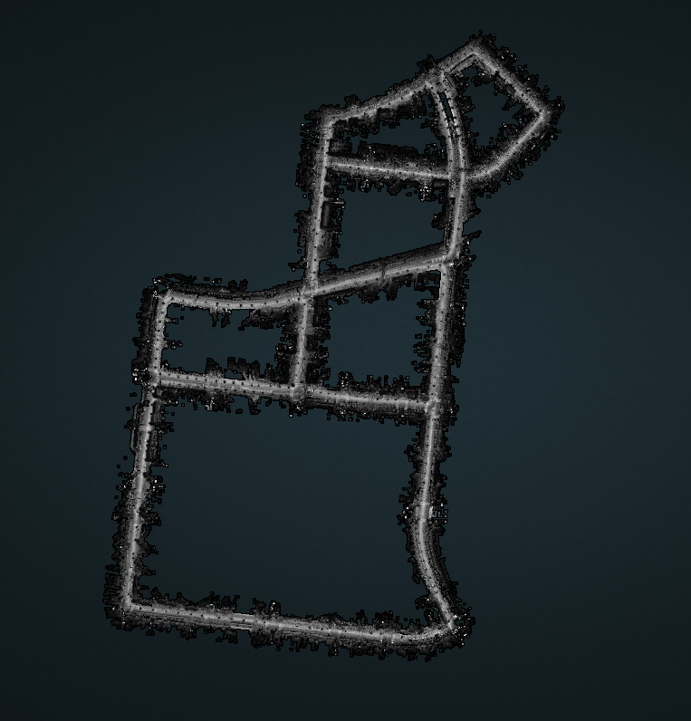
To thoroughly validate the method, both scenes with rich semantic information (such as public roads) and places without semantic information (such as residential areas and very narrow roads in industrial parks) were selected. One of the sites is shown below:
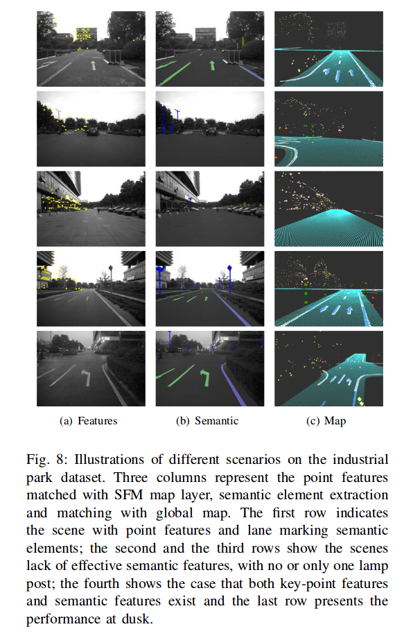
Matched feature points, semantic elements and ground points under different conditions.
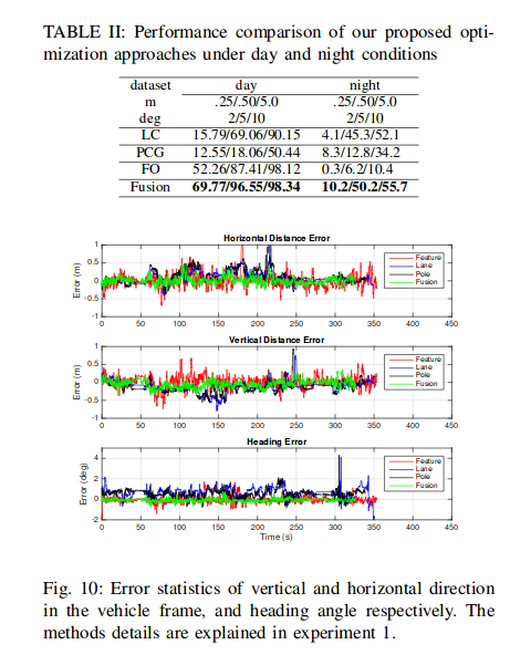
The accuracy is evaluated by dividing it into several separate modules:
- LC (lane curb): optimization using only lane and curb
- PCG (Pole-Curb-Ground): optimization using pole, curb and ground points
- FO (feature only): using only key-point features
- Fusion: the fusion method
Accuracy and robustness:
Localization effectiveness in different scenes:
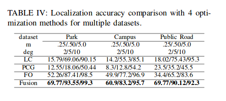
With 52 km of test data, different methods are suited to different scenes respectively; fusion is better.
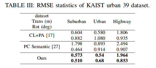
Experiments on the KAIST dataset
Experiments are conducted on the KAIST urban39 data, whose scenes include urban, highway and suburban. The RMSE of the translation and rotation results is shown in the table below:
megivll: pole-based localization, decoupling the estimation of translation and rotation.
Chalmers University of Technology: semantics-based particle-filter localization.
- Runtime analysis
Real-time pose estimation for 10 Hz imagery; timing statistics:
- Semantic segmentation (15 ms)
- Feature-point extraction (< 10 ms)
- Optimization (20 ms)
Comments